OneSidedFrequentistUpperLimitWithBands.C File Reference

Detailed Description

OneSidedFrequentistUpperLimitWithBands

This is a standard demo that can be used with any ROOT file prepared in the standard way. You specify:

• name for input ROOT file
• name of workspace inside ROOT file that holds model and data
• name of ModelConfig that specifies details for calculator tools
• name of dataset

With default parameters the macro will attempt to run the standard hist2workspace example and read the ROOT file that it produces.

The first ~100 lines define a new test statistic, then the main macro starts. You may want to control:

double confidenceLevel=0.95;
int nPointsToScan = 12;
int nToyMC = 150;

This uses a modified version of the profile likelihood ratio as a test statistic for upper limits (eg. test stat = 0 if muhat>mu).

Based on the observed data, one defines a set of parameter points to be tested based on the value of the parameter of interest and the conditional MLE (eg. profiled) values of the nuisance parameters.

At each parameter point, pseudo-experiments are generated using this fixed reference model and then the test statistic is evaluated. Note, the nuisance parameters are floating in the fits. For each point, the threshold that defines the 95% acceptance region is found. This forms a "Confidence Belt".

After constructing the confidence belt, one can find the confidence interval for any particular dataset by finding the intersection of the observed test statistic and the confidence belt. First this is done on the observed data to get an observed 1-sided upper limt.

Finally, there expected limit and bands (from background-only) are formed by generating background-only data and finding the upper limit. This is done by hand for now, will later be part of the RooStats tools.

On a technical note, this technique is NOT the Feldman-Cousins technique, because that is a 2-sided interval BY DEFINITION. However, like the Feldman-Cousins technique this is a Neyman-Construction. For technical reasons the easiest way to implement this right now is to use the FeldmanCousins tool and then change the test statistic that it is using.

Building the confidence belt can be computationally expensive. Once it is built, one could save it to a file and use it in a separate step.

We can use PROOF to speed things along in parallel, however, the test statistic has to be installed on the workers so either turn off PROOF or include the modified test statistic in your $ROOTSYS/roofit/roostats/inc directory, add the additional line to the LinkDef.h file, and recompile root.

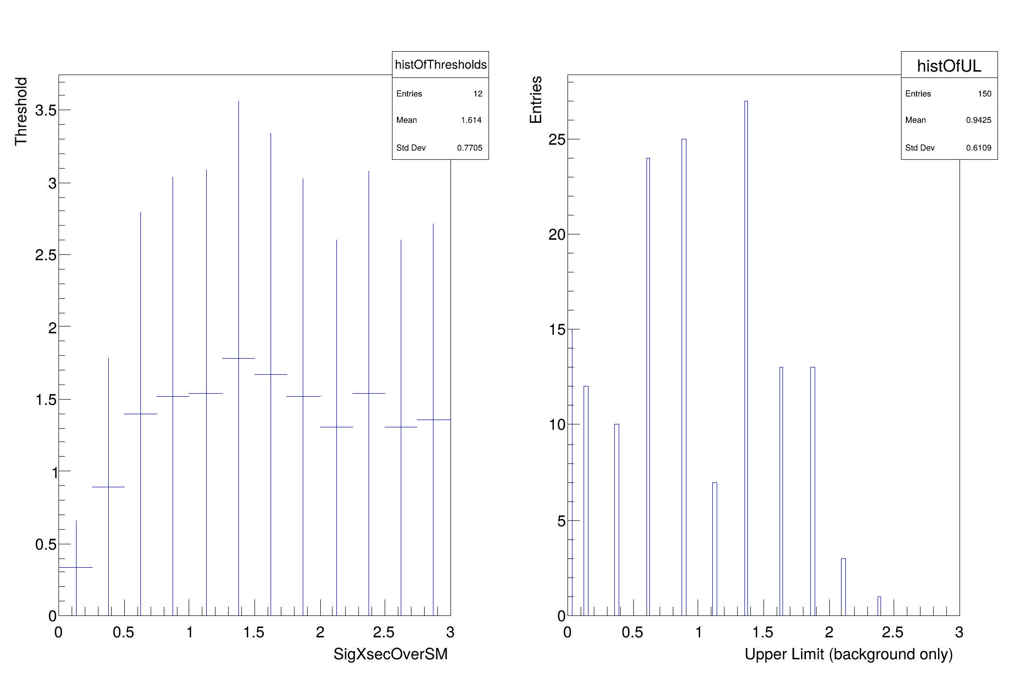
Note, if you have a boundary on the parameter of interest (eg. cross-section) the threshold on the one-sided test statistic starts off very small because we are only including downward fluctuations. You can see the threshold in these printouts:

[#0] PROGRESS:Generation -- generated toys: 500 / 999
NeymanConstruction: Prog: 12/50 total MC = 39 this test stat = 0
 SigXsecOverSM=0.69 alpha_syst1=0.136515 alpha_syst3=0.425415 beta_syst2=1.08496 [-1e+30, 0.011215]  in interval = 1

this tells you the values of the parameters being used to generate the pseudo-experiments and the threshold in this case is 0.011215. One would expect for 95% that the threshold would be ~1.35 once the cross-section is far enough away from 0 that it is essentially unaffected by the boundary. As one reaches the last points in the scan, the threshold starts to get artificially high. This is because the range of the parameter in the fit is the same as the range in the scan. In the future, these should be independently controlled, but they are not now. As a result the ~50% of pseudo-experiments that have an upward fluctuation end up with muhat = muMax. Because of this, the upper range of the parameter should be well above the expected upper limit... but not too high or one will need a very large value of nPointsToScan to resolve the relevant region. This can be improved, but this is the first version of this script.

Important note: when the model includes external constraint terms, like a Gaussian constraint to a nuisance parameter centered around some nominal value there is a subtlety. The asymptotic results are all based on the assumption that all the measurements fluctuate... including the nominal values from auxiliary measurements. If these do not fluctuate, this corresponds to an "conditional ensemble". The result is that the distribution of the test statistic can become very non-chi^2. This results in thresholds that become very large. This can be seen in the following thought experiment. Say the model is $Pois(N|s+b)G(b0|b,sigma)$ where $G(b0|b,sigma)$ is the external constraint and b0 is 100. If N is also 100 then the profiled value of b given s is going to be some trade off between 100-s and b0. If sigma is $\sqrt{(}N)$, then the profiled value of b is probably 100 - s/2 So for s=60 we are going to have a profiled value of b~70. Now when we generate pseudo-experiments for s=60, b=70 we will have N~130 and the average shat will be 30, not 60. In practice, this is only an issue for values of s that are very excluded. For values of s near the 95% limit this should not be a big effect. This can be avoided if the nominal values of the constraints also fluctuate, but that requires that those parameters are RooRealVars in the model. This version does not deal with this issue, but it will be addressed in a future version.

 
FeldmanCousins: ntoys per point = 499
FeldmanCousins: nEvents per toy will fluctuate about  expectation
will use global observables for unconditional ensemble
RooArgSet:: = (nominalLumi,nom_alpha_syst1,nom_alpha_syst2,nom_alpha_syst3,nom_gamma_stat_channel1_bin_0,nom_gamma_stat_channel1_bin_1)
 
=== Using the following for ModelConfig ===
Observables:             RooArgSet:: = (obs_x_channel1,channelCat)
Parameters of Interest:  RooArgSet:: = (SigXsecOverSM)
Nuisance Parameters:     RooArgSet:: = (alpha_syst2,alpha_syst3,gamma_stat_channel1_bin_0,gamma_stat_channel1_bin_1)
Global Observables:      RooArgSet:: = (nominalLumi,nom_alpha_syst1,nom_alpha_syst2,nom_alpha_syst3,nom_gamma_stat_channel1_bin_0,nom_gamma_stat_channel1_bin_1)
PDF:                     RooSimultaneous::simPdf[ indexCat=channelCat channel1=model_channel1 ] = 0.190787
 
FeldmanCousins: Model has nuisance parameters, will do profile construction
FeldmanCousins: # points to test = 12
lookup index = 0
NeymanConstruction: Prog: 1/12 total MC = 499 this test stat = 0
 SigXsecOverSM=0.125 alpha_syst2=0.61993 alpha_syst3=0.233335 gamma_stat_channel1_bin_0=1.03212 gamma_stat_channel1_bin_1=1.04741 [-inf, 0.329584]  in interval = 1
 
NeymanConstruction: Prog: 2/12 total MC = 499 this test stat = 0
 SigXsecOverSM=0.375 alpha_syst2=0.458263 alpha_syst3=0.183235 gamma_stat_channel1_bin_0=1.02329 gamma_stat_channel1_bin_1=1.03422 [-inf, 0.888912]  in interval = 1
 
NeymanConstruction: Prog: 3/12 total MC = 499 this test stat = 0
 SigXsecOverSM=0.625 alpha_syst2=0.292479 alpha_syst3=0.126723 gamma_stat_channel1_bin_0=1.01484 gamma_stat_channel1_bin_1=1.02374 [-inf, 1.39758]  in interval = 1
 
NeymanConstruction: Prog: 4/12 total MC = 499 this test stat = 0
 SigXsecOverSM=0.875 alpha_syst2=0.130655 alpha_syst3=0.0953602 gamma_stat_channel1_bin_0=1.00646 gamma_stat_channel1_bin_1=1.01288 [-inf, 1.51992]  in interval = 1
 
NeymanConstruction: Prog: 5/12 total MC = 499 this test stat = 0.000124169
 SigXsecOverSM=1.125 alpha_syst2=-0.0146474 alpha_syst3=0.0173394 gamma_stat_channel1_bin_0=0.999267 gamma_stat_channel1_bin_1=1.003 [-inf, 1.54198]  in interval = 1
 
NeymanConstruction: Prog: 6/12 total MC = 499 this test stat = 0.0913576
 SigXsecOverSM=1.375 alpha_syst2=-0.15078 alpha_syst3=-0.0572169 gamma_stat_channel1_bin_0=0.99238 gamma_stat_channel1_bin_1=0.993157 [-inf, 1.78377]  in interval = 1
 
NeymanConstruction: Prog: 7/12 total MC = 499 this test stat = 0.349003
 SigXsecOverSM=1.625 alpha_syst2=-0.294555 alpha_syst3=-0.0932947 gamma_stat_channel1_bin_0=0.985516 gamma_stat_channel1_bin_1=0.983192 [-inf, 1.66921]  in interval = 1
 
NeymanConstruction: Prog: 8/12 total MC = 499 this test stat = 0.767692
 SigXsecOverSM=1.875 alpha_syst2=-0.424297 alpha_syst3=-0.146312 gamma_stat_channel1_bin_0=0.979248 gamma_stat_channel1_bin_1=0.973447 [-inf, 1.5144]  in interval = 1
 
NeymanConstruction: Prog: 9/12 total MC = 499 this test stat = 1.34313
 SigXsecOverSM=2.125 alpha_syst2=-0.546305 alpha_syst3=-0.198112 gamma_stat_channel1_bin_0=0.973364 gamma_stat_channel1_bin_1=0.963869 [-inf, 1.30266]  in interval = 0
 
NeymanConstruction: Prog: 10/12 total MC = 499 this test stat = 2.07172
 SigXsecOverSM=2.375 alpha_syst2=-0.66027 alpha_syst3=-0.248685 gamma_stat_channel1_bin_0=0.967841 gamma_stat_channel1_bin_1=0.954463 [-inf, 1.5387]  in interval = 0
 
NeymanConstruction: Prog: 11/12 total MC = 499 this test stat = 2.9476
 SigXsecOverSM=2.625 alpha_syst2=-0.766369 alpha_syst3=-0.29799 gamma_stat_channel1_bin_0=0.962657 gamma_stat_channel1_bin_1=0.945235 [-inf, 1.30108]  in interval = 0
 
NeymanConstruction: Prog: 12/12 total MC = 499 this test stat = 3.96711
 SigXsecOverSM=2.875 alpha_syst2=-0.865262 alpha_syst3=-0.345965 gamma_stat_channel1_bin_0=0.95779 gamma_stat_channel1_bin_1=0.936192 [-inf, 1.35603]  in interval = 0
 
[#1] INFO:Eval -- 8 points in interval
 
95% interval on SigXsecOverSM is : [0.125, 1.875] 
[#1] INFO:Minimization -- p.d.f. provides expected number of events, including extended term in likelihood.
[#1] INFO:Minimization --  Including the following constraint terms in minimization: (lumiConstraint,alpha_syst1Constraint,alpha_syst2Constraint,alpha_syst3Constraint,gamma_stat_channel1_bin_0_constraint,gamma_stat_channel1_bin_1_constraint)
[#1] INFO:Minimization -- The global observables are not defined , normalize constraints with respect to the parameters (Lumi,SigXsecOverSM,alpha_syst1,alpha_syst2,alpha_syst3,gamma_stat_channel1_bin_0,gamma_stat_channel1_bin_1)
[#1] INFO:Fitting -- RooAbsPdf::fitTo(simPdf) fixing normalization set for coefficient determination to observables in data
[#1] INFO:Fitting -- using CPU computation library compiled with -mavx512
[#1] INFO:Minimization -- RooProfileLL::evaluate(RooEvaluatorWrapper_Profile[SigXsecOverSM]) Creating instance of MINUIT
[#1] INFO:Fitting -- RooAddition::defaultErrorLevel(nll_simPdf_obsData) Summation contains a RooNLLVar, using its error level
[#1] INFO:Minimization -- RooProfileLL::evaluate(RooEvaluatorWrapper_Profile[SigXsecOverSM]) determining minimum likelihood for current configurations w.r.t all observable
[#1] INFO:Minimization -- RooProfileLL::evaluate(RooEvaluatorWrapper_Profile[SigXsecOverSM]) minimum found at (SigXsecOverSM=1.12136)
.
Will use these parameter points to generate pseudo data for bkg only
  1) 0x964afe0 RooRealVar::               alpha_syst2 = 0.710958 +/- 0.914123  L(-5 - 5)  "alpha_syst2"
  2) 0x964b4f0 RooRealVar::               alpha_syst3 = 0.261478 +/- 0.929174  L(-5 - 5)  "alpha_syst3"
  3) 0x964ba50 RooRealVar:: gamma_stat_channel1_bin_0 = 1.03677 +/- 0.0462911  L(0 - 1.25)  "gamma_stat_channel1_bin_0"
  4) 0x964bfb0 RooRealVar:: gamma_stat_channel1_bin_1 = 1.05318 +/- 0.0761263  L(0 - 1.5)  "gamma_stat_channel1_bin_1"
  5) 0x964c510 RooRealVar::             SigXsecOverSM = 0 +/- 0  L(0 - 3) B(12)  "SigXsecOverSM"
-2 sigma  band 3.79538e-316
-1 sigma  band 0.105 [Power Constraint)]
median of band 0.855
+1 sigma  band 1.605
+2 sigma  band 2.085
 
observed 95% upper-limit 1.875
CLb strict [P(toy>obs|0)] for observed 95% upper-limit 0.966667
CLb inclusive [P(toy>=obs|0)] for observed 95% upper-limit 0.966667

 
#include "TFile.h"
#include "TROOT.h"
#include "TH1F.h"
#include "TCanvas.h"
#include "TSystem.h"
 
#include "RooWorkspace.h"
#include "RooSimultaneous.h"
#include "RooAbsData.h"
 
#include "RooStats/ModelConfig.h"
#include "RooStats/FeldmanCousins.h"
#include "RooStats/ToyMCSampler.h"
#include "RooStats/PointSetInterval.h"
#include "RooStats/ConfidenceBelt.h"
 
#include "RooStats/RooStatsUtils.h"
#include "RooStats/ProfileLikelihoodTestStat.h"
 
using namespace RooFit;
using namespace RooStats;
 
bool useProof = false; // flag to control whether to use Proof
int nworkers = 0;      // number of workers (default use all available cores)
 
// -------------------------------------------------------
// The actual macro
 
void OneSidedFrequentistUpperLimitWithBands(const char *infile = "", const char *workspaceName = "combined",
                                            const char *modelConfigName = "ModelConfig",
                                            const char *dataName = "obsData")
{
 
   double confidenceLevel = 0.95;
   int nPointsToScan = 12;
   int nToyMC = 150;
 
   // -------------------------------------------------------
   // First part is just to access a user-defined file
   // or create the standard example file if it doesn't exist
   const char *filename = "";
   if (!strcmp(infile, "")) {
      filename = "results/example_combined_GaussExample_model.root";
      bool fileExist = !gSystem->AccessPathName(filename); // note opposite return code
      // if file does not exists generate with histfactory
      if (!fileExist) {
         // Normally this would be run on the command line
         cout << "will run standard hist2workspace example" << endl;
         gROOT->ProcessLine(".! prepareHistFactory .");
         gROOT->ProcessLine(".! hist2workspace config/example.xml");
         cout << "\n\n---------------------" << endl;
         cout << "Done creating example input" << endl;
         cout << "---------------------\n\n" << endl;
      }
 
   } else
      filename = infile;
 
   // Try to open the file
   TFile *file = TFile::Open(filename);
 
   // if input file was specified byt not found, quit
   if (!file) {
      cout << "StandardRooStatsDemoMacro: Input file " << filename << " is not found" << endl;
      return;
   }
 
   // -------------------------------------------------------
   // Now get the data and workspace
 
   // get the workspace out of the file
   RooWorkspace *w = (RooWorkspace *)file->Get(workspaceName);
   if (!w) {
      cout << "workspace not found" << endl;
      return;
   }
 
   // get the modelConfig out of the file
   ModelConfig *mc = (ModelConfig *)w->obj(modelConfigName);
 
   // get the modelConfig out of the file
   RooAbsData *data = w->data(dataName);
 
   // make sure ingredients are found
   if (!data || !mc) {
      w->Print();
      cout << "data or ModelConfig was not found" << endl;
      return;
   }
 
   // -------------------------------------------------------
   // Now get the POI for convenience
   // you may want to adjust the range of your POI
 
   RooRealVar *firstPOI = (RooRealVar *)mc->GetParametersOfInterest()->first();
   /*  firstPOI->setMin(0);*/
   /*  firstPOI->setMax(10);*/
 
   // --------------------------------------------
   // Create and use the FeldmanCousins tool
   // to find and plot the 95% confidence interval
   // on the parameter of interest as specified
   // in the model config
   // REMEMBER, we will change the test statistic
   // so this is NOT a Feldman-Cousins interval
   FeldmanCousins fc(*data, *mc);
   fc.SetConfidenceLevel(confidenceLevel);
   fc.AdditionalNToysFactor(
      0.5); // degrade/improve sampling that defines confidence belt: in this case makes the example faster
   /*  fc.UseAdaptiveSampling(true); // speed it up a bit, don't use for expected limits*/
   fc.SetNBins(nPointsToScan); // set how many points per parameter of interest to scan
   fc.CreateConfBelt(true);    // save the information in the belt for plotting
 
   // -------------------------------------------------------
   // Feldman-Cousins is a unified limit by definition
   // but the tool takes care of a few things for us like which values
   // of the nuisance parameters should be used to generate toys.
   // so let's just change the test statistic and realize this is
   // no longer "Feldman-Cousins" but is a fully frequentist Neyman-Construction.
   /*  ProfileLikelihoodTestStatModified onesided(*mc->GetPdf());*/
   /*  fc.GetTestStatSampler()->SetTestStatistic(&onesided);*/
   /* ((ToyMCSampler*) fc.GetTestStatSampler())->SetGenerateBinned(true); */
   ToyMCSampler *toymcsampler = (ToyMCSampler *)fc.GetTestStatSampler();
   ProfileLikelihoodTestStat *testStat = dynamic_cast<ProfileLikelihoodTestStat *>(toymcsampler->GetTestStatistic());
   testStat->SetOneSided(true);
 
   // Since this tool needs to throw toy MC the PDF needs to be
   // extended or the tool needs to know how many entries in a dataset
   // per pseudo experiment.
   // In the 'number counting form' where the entries in the dataset
   // are counts, and not values of discriminating variables, the
   // datasets typically only have one entry and the PDF is not
   // extended.
   if (!mc->GetPdf()->canBeExtended()) {
      if (data->numEntries() == 1)
         fc.FluctuateNumDataEntries(false);
      else
         cout << "Not sure what to do about this model" << endl;
   }
 
   // We can use PROOF to speed things along in parallel
   // However, the test statistic has to be installed on the workers
   // so either turn off PROOF or include the modified test statistic
   // in your `$ROOTSYS/roofit/roostats/inc` directory,
   // add the additional line to the LinkDef.h file,
   // and recompile root.
   if (useProof) {
      ProofConfig pc(*w, nworkers, "", false);
      toymcsampler->SetProofConfig(&pc); // enable proof
   }
 
   if (mc->GetGlobalObservables()) {
      cout << "will use global observables for unconditional ensemble" << endl;
      mc->GetGlobalObservables()->Print();
      toymcsampler->SetGlobalObservables(*mc->GetGlobalObservables());
   }
 
   // Now get the interval
   PointSetInterval *interval = fc.GetInterval();
   ConfidenceBelt *belt = fc.GetConfidenceBelt();
 
   // print out the interval on the first Parameter of Interest
   cout << "\n95% interval on " << firstPOI->GetName() << " is : [" << interval->LowerLimit(*firstPOI) << ", "
        << interval->UpperLimit(*firstPOI) << "] " << endl;
 
   // get observed UL and value of test statistic evaluated there
   RooArgSet tmpPOI(*firstPOI);
   double observedUL = interval->UpperLimit(*firstPOI);
   firstPOI->setVal(observedUL);
   double obsTSatObsUL = fc.GetTestStatSampler()->EvaluateTestStatistic(*data, tmpPOI);
 
   // Ask the calculator which points were scanned
   RooDataSet *parameterScan = (RooDataSet *)fc.GetPointsToScan();
   RooArgSet *tmpPoint;
 
   // make a histogram of parameter vs. threshold
   TH1F *histOfThresholds =
      new TH1F("histOfThresholds", "", parameterScan->numEntries(), firstPOI->getMin(), firstPOI->getMax());
   histOfThresholds->GetXaxis()->SetTitle(firstPOI->GetName());
   histOfThresholds->GetYaxis()->SetTitle("Threshold");
 
   // loop through the points that were tested and ask confidence belt
   // what the upper/lower thresholds were.
   // For FeldmanCousins, the lower cut off is always 0
   for (Int_t i = 0; i < parameterScan->numEntries(); ++i) {
      tmpPoint = (RooArgSet *)parameterScan->get(i)->clone("temp");
      // cout <<"get threshold"<<endl;
      double arMax = belt->GetAcceptanceRegionMax(*tmpPoint);
      double poiVal = tmpPoint->getRealValue(firstPOI->GetName());
      histOfThresholds->Fill(poiVal, arMax);
   }
   TCanvas *c1 = new TCanvas();
   c1->Divide(2);
   c1->cd(1);
   histOfThresholds->SetMinimum(0);
   histOfThresholds->Draw();
   c1->cd(2);
 
   // -------------------------------------------------------
   // Now we generate the expected bands and power-constraint
 
   // First: find parameter point for mu=0, with conditional MLEs for nuisance parameters
   std::unique_ptr<RooAbsReal> nll{mc->GetPdf()->createNLL(*data)};
   std::unique_ptr<RooAbsReal> profile{nll->createProfile(*mc->GetParametersOfInterest())};
   firstPOI->setVal(0.);
   profile->getVal(); // this will do fit and set nuisance parameters to profiled values
   RooArgSet *poiAndNuisance = new RooArgSet();
   if (mc->GetNuisanceParameters())
      poiAndNuisance->add(*mc->GetNuisanceParameters());
   poiAndNuisance->add(*mc->GetParametersOfInterest());
   w->saveSnapshot("paramsToGenerateData", *poiAndNuisance);
   RooArgSet *paramsToGenerateData = (RooArgSet *)poiAndNuisance->snapshot();
   cout << "\nWill use these parameter points to generate pseudo data for bkg only" << endl;
   paramsToGenerateData->Print("v");
 
   RooArgSet unconditionalObs;
   unconditionalObs.add(*mc->GetObservables());
   unconditionalObs.add(*mc->GetGlobalObservables()); // comment this out for the original conditional ensemble
 
   double CLb = 0;
   double CLbinclusive = 0;
 
   // Now we generate background only and find distribution of upper limits
   TH1F *histOfUL = new TH1F("histOfUL", "", 100, 0, firstPOI->getMax());
   histOfUL->GetXaxis()->SetTitle("Upper Limit (background only)");
   histOfUL->GetYaxis()->SetTitle("Entries");
   for (int imc = 0; imc < nToyMC; ++imc) {
 
      // set parameters back to values for generating pseudo data
      //    cout << "\n get current nuis, set vals, print again" << endl;
      w->loadSnapshot("paramsToGenerateData");
      //    poiAndNuisance->Print("v");
 
      std::unique_ptr<RooDataSet> toyData;
      // now generate a toy dataset
      if (!mc->GetPdf()->canBeExtended()) {
         if (data->numEntries() == 1)
            toyData = std::unique_ptr<RooDataSet>{mc->GetPdf()->generate(*mc->GetObservables(), 1)};
         else
            cout << "Not sure what to do about this model" << endl;
      } else {
         //      cout << "generating extended dataset"<<endl;
         toyData = std::unique_ptr<RooDataSet>{mc->GetPdf()->generate(*mc->GetObservables(), Extended())};
      }
 
      // generate global observables
      // need to be careful for simpdf
      //    RooDataSet* globalData = mc->GetPdf()->generate(*mc->GetGlobalObservables(),1);
 
      RooSimultaneous *simPdf = dynamic_cast<RooSimultaneous *>(mc->GetPdf());
      if (!simPdf) {
         std::unique_ptr<RooDataSet> one{mc->GetPdf()->generate(*mc->GetGlobalObservables(), 1)};
         const RooArgSet *values = one->get();
         std::unique_ptr<RooArgSet> allVars{mc->GetPdf()->getVariables()};
         allVars->assign(*values);
      } else {
 
         // try fix for sim pdf
         for (auto const& tt : simPdf->indexCat()) {
            auto const& catName = tt.first;
 
            // Get pdf associated with state from simpdf
            RooAbsPdf *pdftmp = simPdf->getPdf(catName.c_str());
 
            // Generate only global variables defined by the pdf associated with this state
            std::unique_ptr<RooArgSet> globtmp{pdftmp->getObservables(*mc->GetGlobalObservables())};
            std::unique_ptr<RooDataSet> tmp{pdftmp->generate(*globtmp, 1)};
 
            // Transfer values to output placeholder
            globtmp->assign(*tmp->get(0));
         }
      }
 
      //    globalData->Print("v");
      //    unconditionalObs = *globalData->get();
      //    mc->GetGlobalObservables()->Print("v");
      //    delete globalData;
      //    cout << "toy data = " << endl;
      //    toyData->get()->Print("v");
 
      // get test stat at observed UL in observed data
      firstPOI->setVal(observedUL);
      double toyTSatObsUL = fc.GetTestStatSampler()->EvaluateTestStatistic(*toyData, tmpPOI);
      //    toyData->get()->Print("v");
      //    cout <<"obsTSatObsUL " <<obsTSatObsUL << "toyTS " << toyTSatObsUL << endl;
      if (obsTSatObsUL < toyTSatObsUL) // not sure about <= part yet
         CLb += (1.) / nToyMC;
      if (obsTSatObsUL <= toyTSatObsUL) // not sure about <= part yet
         CLbinclusive += (1.) / nToyMC;
 
      // loop over points in belt to find upper limit for this toy data
      double thisUL = 0;
      for (Int_t i = 0; i < parameterScan->numEntries(); ++i) {
         tmpPoint = (RooArgSet *)parameterScan->get(i)->clone("temp");
         double arMax = belt->GetAcceptanceRegionMax(*tmpPoint);
         firstPOI->setVal(tmpPoint->getRealValue(firstPOI->GetName()));
         //   double thisTS = profile->getVal();
         double thisTS = fc.GetTestStatSampler()->EvaluateTestStatistic(*toyData, tmpPOI);
 
         //   cout << "poi = " << firstPOI->getVal()
         // << " max is " << arMax << " this profile = " << thisTS << endl;
         //      cout << "thisTS = " << thisTS<<endl;
         if (thisTS <= arMax) {
            thisUL = firstPOI->getVal();
         } else {
            break;
         }
      }
 
      /*
      // loop over points in belt to find upper limit for this toy data
      double thisUL = 0;
      for(Int_t i=0; i<histOfThresholds->GetNbinsX(); ++i){
         tmpPoint = (RooArgSet*) parameterScan->get(i)->clone("temp");
         cout <<"----------------  "<<i<<endl;
         tmpPoint->Print("v");
         cout << "from hist " << histOfThresholds->GetBinCenter(i+1) <<endl;
         double arMax = histOfThresholds->GetBinContent(i+1);
         // cout << " threshold from Hist = aMax " << arMax<<endl;
         // double arMax2 = belt->GetAcceptanceRegionMax(*tmpPoint);
         // cout << "from scan arMax2 = "<< arMax2 << endl; // not the same due to TH1F not TH1D
         // cout << "scan - hist" << arMax2-arMax << endl;
         firstPOI->setVal( histOfThresholds->GetBinCenter(i+1));
         //   double thisTS = profile->getVal();
         double thisTS = fc.GetTestStatSampler()->EvaluateTestStatistic(*toyData,tmpPOI);
 
         //   cout << "poi = " << firstPOI->getVal()
         // << " max is " << arMax << " this profile = " << thisTS << endl;
         //      cout << "thisTS = " << thisTS<<endl;
 
         // NOTE: need to add a small epsilon term for single precision vs. double precision
         if(thisTS<=arMax + 1e-7){
            thisUL = firstPOI->getVal();
         } else{
            break;
         }
      }
      */
 
      histOfUL->Fill(thisUL);
 
      // for few events, data is often the same, and UL is often the same
      //    cout << "thisUL = " << thisUL<<endl;
   }
   histOfUL->Draw();
   c1->SaveAs("one-sided_upper_limit_output.pdf");
 
   // if you want to see a plot of the sampling distribution for a particular scan point:
   /*
   SamplingDistPlot sampPlot;
   int indexInScan = 0;
   tmpPoint = (RooArgSet*) parameterScan->get(indexInScan)->clone("temp");
   firstPOI->setVal( tmpPoint->getRealValue(firstPOI->GetName()) );
   toymcsampler->SetParametersForTestStat(tmpPOI);
   SamplingDistribution* samp = toymcsampler->GetSamplingDistribution(*tmpPoint);
   sampPlot.AddSamplingDistribution(samp);
   sampPlot.Draw();
      */
 
   // Now find bands and power constraint
   Double_t *bins = histOfUL->GetIntegral();
   TH1F *cumulative = (TH1F *)histOfUL->Clone("cumulative");
   cumulative->SetContent(bins);
   double band2sigDown, band1sigDown, bandMedian, band1sigUp, band2sigUp;
   for (int i = 1; i <= cumulative->GetNbinsX(); ++i) {
      if (bins[i] < RooStats::SignificanceToPValue(2))
         band2sigDown = cumulative->GetBinCenter(i);
      if (bins[i] < RooStats::SignificanceToPValue(1))
         band1sigDown = cumulative->GetBinCenter(i);
      if (bins[i] < 0.5)
         bandMedian = cumulative->GetBinCenter(i);
      if (bins[i] < RooStats::SignificanceToPValue(-1))
         band1sigUp = cumulative->GetBinCenter(i);
      if (bins[i] < RooStats::SignificanceToPValue(-2))
         band2sigUp = cumulative->GetBinCenter(i);
   }
   cout << "-2 sigma  band " << band2sigDown << endl;
   cout << "-1 sigma  band " << band1sigDown << " [Power Constraint)]" << endl;
   cout << "median of band " << bandMedian << endl;
   cout << "+1 sigma  band " << band1sigUp << endl;
   cout << "+2 sigma  band " << band2sigUp << endl;
 
   // print out the interval on the first Parameter of Interest
   cout << "\nobserved 95% upper-limit " << interval->UpperLimit(*firstPOI) << endl;
   cout << "CLb strict [P(toy>obs|0)] for observed 95% upper-limit " << CLb << endl;
   cout << "CLb inclusive [P(toy>=obs|0)] for observed 95% upper-limit " << CLbinclusive << endl;
}

Authors

Kyle Cranmer, Haichen Wang, Daniel Whiteson

Definition in file OneSidedFrequentistUpperLimitWithBands.C.