Distributions

Some analyses want to check theory predictions that exist as a function definition. Others want to use a distribution from a histogram in another step of the analysis. But histograms have bin steps by nature instead of being smooth, and they have bumps / fluctuations due to limited statistics (i.e. "not enough data").

So what's needed is a function whose line is "as close as possible" to the histogram counts. I.e. we need a function (that predicts the shape of the histogram) and that we can vary a bit ("free parameters"). Then we search for the best set of parameters, such that the function resembles the histogram.

That's fitting.

Fitting in Practice

As often with ROOT, you can use a GUI element (the fit panel, available through the menu in "Tools", "Fit Panel", or on the prompt (TH1::Fit()). Let's use the fit panel!

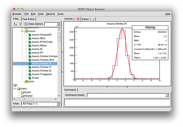
First, we draw the distribution of the vertex position along X for all muons. Do that into a histogram that has 20 bins and runs from -10 to +10. Now open the fit panel and click the histogram. We want to fit a Gaussian distribution - and hat's already selected by default. Se just press "Fit". Looks good, right? Fit Parameters

As mentioned before, fitting means finding the optimal set of parameters. In the menu, select "Options", "Fit Parameters" (and resize the statistics box to make its content readable). You will see the values that the minimizer has found optimal, for instance it chose 1.2 as the mean of the Gaussian and 1.041 as the width.

These values are the crucial ones for physicists: they reduce the large amount of data into just a few parameters, describing the distribution even better than the original histogram. Fitting (or "parametrization") is thus a cornerstone of any physics analysis.