Suppose we do not need unlimited precision on some variable X, but only need to know how many times its value falls between x₁ and x₂, or between x₂ and x₃, etc. In practice, we define a partition of the interval (x₁, x_N+1) by using the N+1 values x₁x₁x_N+1 (that in most applications are equally spaced), and call the i-th bin the interval defined by the pair (x_i, x_i+1). Then, we associate to each bin an integer number n_i, that is the number of times the condition x_ix_i+1 occurs in our data sample about X. In its simplest form, a (1-dimensional) histogram is defined as the collection of the N pairs (1, n₁), (2, n₂), ..., (N, n_N) and it is usually implemented as an array in which the first value of the pair (i, n_i) is the index of the element containing the value n_i.

In ROOT, 1-dimensional histograms are defined by the base class TH1: actual classes inherit from TH1 and implement histograms in which n_i is an integer (for integer types of increasing precision, use TH1C for char variables, TH1S for short, and TH1I for int) or a real number (use TH1F for float and TH1D for double). A ROOT histogram contains much more information than the aforementioned collection of pairs. First, two more bins are added to represent underflow (entries satisfying the condition X x₀) and overflow (i.e. X > x_N). Second, for each bin, two numbers are retained: its entries n_i and the best estimate e_i of the expected fluctuation on n_i. In addition, a number of additional information is stored, like the total number of entries and the sum of all n_i's (i.e. the integral of the histogram), that may be different from the number of entries (for example, a normalized histogram has unit integral but may have any number of entries). In addition to 1-dimensional histograms, ROOT also provides 2- and 3-dimensional histograms. Finally, ROOT histograms contain a very rich set of additional features that are useful for fits or in graphical representation.

In most cases, histograms are used to count the integer number of times a certain quantity has values in any given bin and are saved into a ROOT file, from which it will be fetched later, during data analysis. In this case, the user needs first to create the histogram, then to loop over all events and fill the histogram (incrementing by 1 the correct bin for each event), and finally needs to save it into a TFile. To create a histogram of floats, the TH1F constructor is used: we have to specify the object name, the title (a single string with format "histogram title;horizontal axis title;vertical axis title" in which the axis titles are optional), the number of bins, the minimum and maximum values:

 
TH1F *hmass = new TH1F("hmass", "Mass;mass (kg)", 100, 0, 5);

To increment the bin containing the current value of our float variable x, the TH1::Fill method is used. Data collected from some measurement are usually counted by incrementing the bin content by 1, however different values of the "weight" are also possible.

 
hmass->Fill(x, 1.0); // value, weight = 1 by default

Using the ROOT interpreter, we can play with histograms in several ways, before deciding what to put in our macro. For example,

 
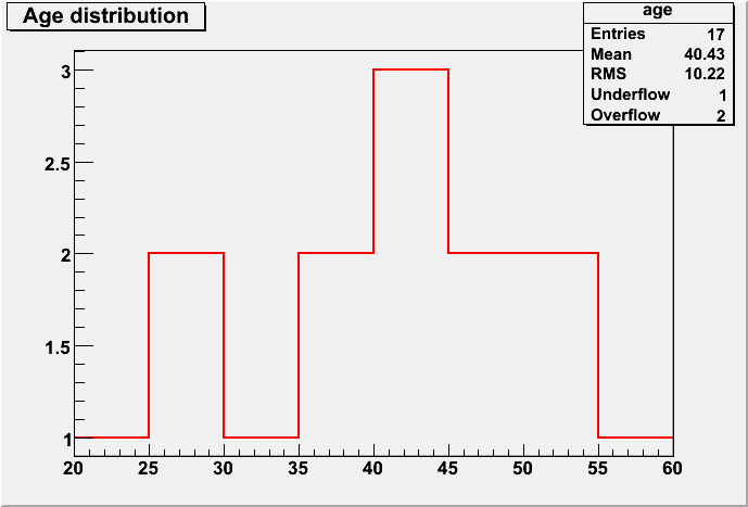
root [] TH1F* hage = new TH1F("age","Age distribution;age (yr)",8,20,60);
root [] float ages[17]={47,35,42,19,56,54,40,39,29,27,30,60,62,23,53,49,42};
root [] for (int i=0; i<17; ++i) hage->Fill(ages[i]);
root [] hage->Draw();
<tcanvas::makedefcanvas>: created default TCanvas with name c1
root [] gStyle->SetOptStat(111111);
root [] hage->SetLineWidth(2);
root [] hage->SetLineColor(2);
root [] hage->Draw();
</tcanvas::makedefcanvas>

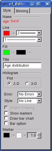
The result is shown below (first plot). We can interactively edit any graphical object in ROOT. For example, we can set a green filling color for the histogram, by right-clicking on it and selecting "DrawPanel" (the editor window shown below pops up), and finally clicking on the small box just below "Fill". The final result is shown in the third panel.

1. Output of last command.
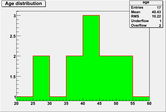3. Final result.	2. Graphical editor.

To save the histogram, the TObject::Write method (inherited by all ROOT classes) is used. The user may use the histogram name or specify a different string for the histogram that will be copied in the currently open TFile.

Histogram errors

ROOT assumes by default that the histogram represents counting of values from stochastically independent measurements (e.g. the outcomes of repeated die throwing), so that it computes the bin fluctuation accordingly to the Poisson distribution: the best estimate of the standard deviation on the observed value n_i of entries in bin i is the square root of n_i. Note that this is not always correct: frequent examples are

• rate histograms: the i-th bin contains the number of events passing cut i and all previous selection criteria. In this case the correct probability distribution is the binomial distribution and the correct standard deviation should be computed by the user (it can also be saved into the histogram itself, for future use). When n_i is not too small, the binomial distribution is well approximated by the Poisson distribution, so that the ROOT default is acceptable in most cases (but not for all bins!). The TH1::Divide(...) method has the option "B" for binomial division, but the best error estimation in this case is provided by TGraphAsymmErrors::BayesDivide() method (which is not as easy to understand ^_^' );
• histograms computed using other histograms, for example by adding or dividing them bin by bin: ROOT assumes that the input histograms have the correct standard deviations and correctly computes the final ones. The user should make sure that the input histograms have correct errors;
• histograms that do not represent value counting from stochastically independent random processes: for each specific case, the user should take care of computing and saving, via TH1::SetBinError(...), the correct standard deviations.

A more detailed (but still concise) review of ROOT histograms is provided by the How to use the histogram classes document.