 |
ROOT 6.14/05 Reference Guide |
| |
ROOT 6.14/05 Reference Guide |
The histogram painter class.
Implements all histograms' drawing's options.
Histograms are drawn via the THistPainter class. Each histogram has a pointer to its own painter (to be usable in a multithreaded program). When the canvas has to be redrawn, the Paint function of each objects in the pad is called. In case of histograms, TH1::Paint invokes directly THistPainter::Paint.
To draw a histogram h it is enough to do:
h->Draw();
h can be of any kind: 1D, 2D or 3D. To choose how the histogram will be drawn, the Draw() method can be invoked with an option. For instance to draw a 2D histogram as a lego plot it is enough to do:
h->Draw("lego");
THistPainter offers many options to paint 1D, 2D and 3D histograms.
When the Draw() method of a histogram is called for the first time (TH1::Draw), it creates a THistPainter object and saves a pointer to this "painter" as a data member of the histogram. The THistPainter class specializes in the drawing of histograms. It is separated from the histogram so that one can have histograms without the graphics overhead, for example in a batch program. Each histogram having its own painter (rather than a central singleton painter painting all histograms), allows two histograms to be drawn in two threads without overwriting the painter's values.
When a displayed histogram is filled again, there is no need to call the Draw() method again; the image will be refreshed the next time the pad will be updated.
A pad is updated after one of these three actions:
TPad::Update.By default a call to TH1::Draw() clears the pad of all objects before drawing the new image of the histogram. One can use the SAME option to leave the previous display intact and superimpose the new histogram. The same histogram can be drawn with different graphics options in different pads.
When a displayed histogram is deleted, its image is automatically removed from the pad.
To create a copy of the histogram when drawing it, one can use TH1::DrawClone(). This will clone the histogram and allow to change and delete the original one without affecting the clone.
Most options can be concatenated with or without spaces or commas, for example:
h->Draw("E1 SAME");
The options are not case sensitive:
h->Draw("e1 same");
The default drawing option can be set with TH1::SetOption and retrieve using TH1::GetOption:
root [0] h->Draw(); // Draw "h" using the standard histogram representation.
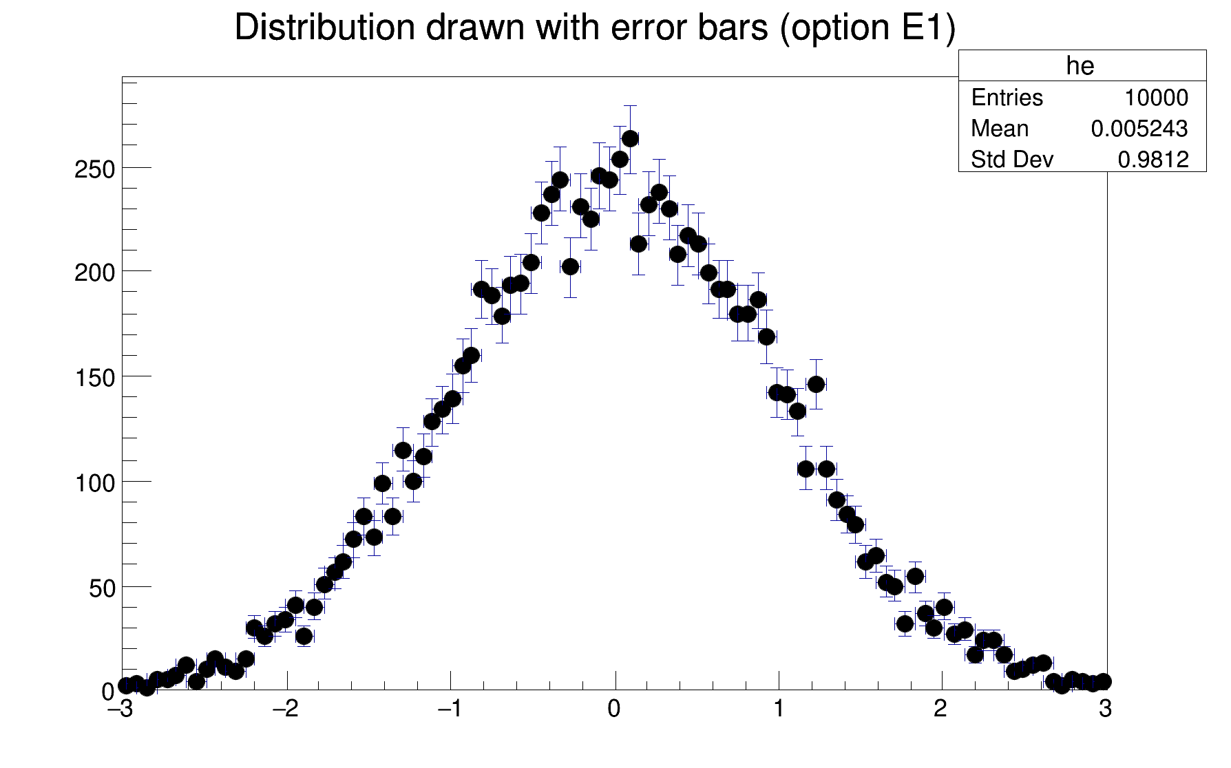
root [1] h->Draw("E"); // Draw "h" using error bars
root [3] h->SetOption("E"); // Change the default drawing option for "h"
root [4] h->Draw(); // Draw "h" using error bars
root [5] h->GetOption(); // Retrieve the default drawing option for "h"
(const Option_t* 0xa3ff948)"E"
| Option | Description |
|---|---|
| " " | Default. |
| "AH" | Draw histogram without axis. "A" can be combined with any drawing option. For instance, "AC" draws the histogram as a smooth Curve without axis. |
| "][" | When this option is selected the first and last vertical lines of the histogram are not drawn. |
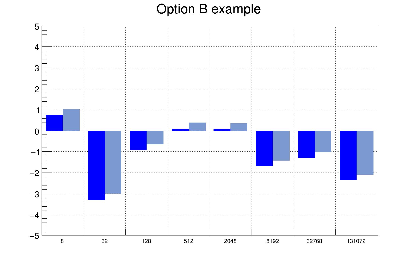
| "B" | Bar chart option. |
| "BAR" | Like option "B", but bars can be drawn with a 3D effect. |
| "HBAR" | Like option "BAR", but bars are drawn horizontally. |
| "C" | Draw a smooth Curve through the histogram bins. |
| "E0" | Draw error bars. Markers are drawn for bins with 0 contents. |
| "E1" | Draw error bars with perpendicular lines at the edges. |
| "E2" | Draw error bars with rectangles. |
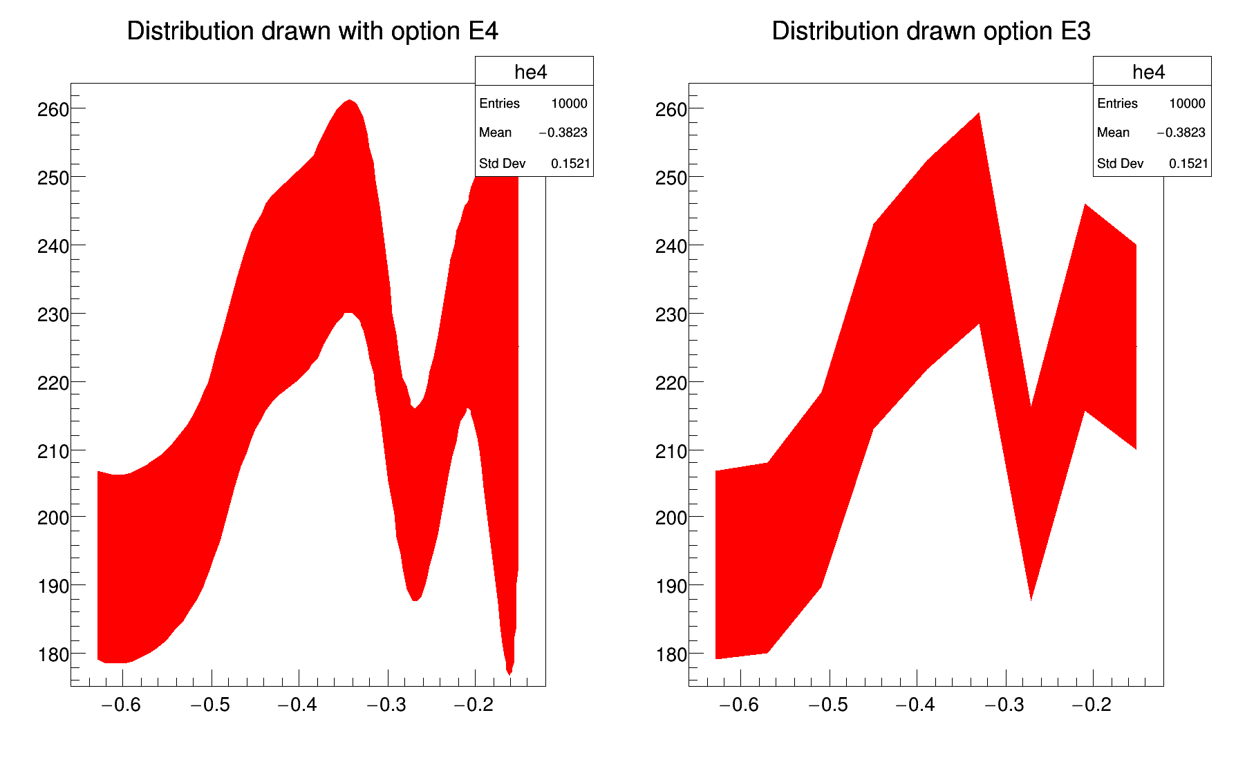
| "E3" | Draw a fill area through the end points of the vertical error bars. |
| "E4" | Draw a smoothed filled area through the end points of the error bars. |
| "E5" | Like E3 but ignore the bins with 0 contents. |
| "E6" | Like E4 but ignore the bins with 0 contents. |
| "X0" | When used with one of the "E" option, it suppress the error bar along X as gStyle->SetErrorX(0) would do. |
| "L" | Draw a line through the bin contents. |
| "P" | Draw current marker at each bin except empty bins. |
| "P0" | Draw current marker at each bin including empty bins. |
| "PIE" | Draw histogram as a Pie Chart. |
| "*H" | Draw histogram with a * at each bin. |
| "LF2" | Draw histogram like with option "L" but with a fill area. Note that "L" draws also a fill area if the hist fill color is set but the fill area corresponds to the histogram contour. |
| Option | Description |
|---|---|
| " " | Default (scatter plot). |
| "ARR" | Arrow mode. Shows gradient between adjacent cells. |
| "BOX" | A box is drawn for each cell with surface proportional to the content's absolute value. A negative content is marked with a X. |
| "BOX1" | A button is drawn for each cell with surface proportional to content's absolute value. A sunken button is drawn for negative values a raised one for positive. |
| "COL" | A box is drawn for each cell with a color scale varying with contents. All the none empty bins are painted. Empty bins are not painted unless some bins have a negative content because in that case the null bins might be not empty. TProfile2D histograms are handled differently because, for this type of 2D histograms, it is possible to know if an empty bin has been filled or not. So even if all the bins' contents are positive some empty bins might be painted. And vice versa, if some bins have a negative content some empty bins might be not painted. |
| "COLZ" | Same as "COL". In addition the color palette is also drawn. |
| "COL2" | Alternative rendering algorithm to "COL". Can significantly improve rendering performance for large, non-sparse 2-D histograms. |
| "COLZ2" | Same as "COL2". In addition the color palette is also drawn. |
| "CANDLE" | Draw a candle plot along X axis. |
| "CANDLEX" | Same as "CANDLE". |
| "CANDLEY" | Draw a candle plot along Y axis. |
| "CANDLEXn" | Draw a candle plot along X axis. Different candle-styles with n from 1 to 6. |
| "CANDLEYn" | Draw a candle plot along Y axis. Different candle-styles with n from 1 to 6. |
| "VIOLIN" | Draw a violin plot along X axis. |
| "VIOLINX" | Same as "VIOLIN". |
| "VIOLINY" | Draw a violin plot along Y axis. |
| "VIOLINXn" | Draw a violin plot along X axis. Different violin-styles with n being 1 or 2. |
| "VIOLINYn" | Draw a violin plot along Y axis. Different violin-styles with n being 1 or 2. |
| "CONT" | Draw a contour plot (same as CONT0). |
| "CONT0" | Draw a contour plot using surface colors to distinguish contours. |
| "CONT1" | Draw a contour plot using line styles to distinguish contours. |
| "CONT2" | Draw a contour plot using the same line style for all contours. |
| "CONT3" | Draw a contour plot using fill area colors. |
| "CONT4" | Draw a contour plot using surface colors (SURF option at theta = 0). |
| "CONT5" | (TGraph2D only) Draw a contour plot using Delaunay triangles. |
| "LIST" | Generate a list of TGraph objects for each contour. |
| "CYL" | Use Cylindrical coordinates. The X coordinate is mapped on the angle and the Y coordinate on the cylinder length. |
| "POL" | Use Polar coordinates. The X coordinate is mapped on the angle and the Y coordinate on the radius. |
| "SPH" | Use Spherical coordinates. The X coordinate is mapped on the latitude and the Y coordinate on the longitude. |
| "PSR" | Use PseudoRapidity/Phi coordinates. The X coordinate is mapped on Phi. |
| "SURF" | Draw a surface plot with hidden line removal. |
| "SURF1" | Draw a surface plot with hidden surface removal. |
| "SURF2" | Draw a surface plot using colors to show the cell contents. |
| "SURF3" | Same as SURF with in addition a contour view drawn on the top. |
| "SURF4" | Draw a surface using Gouraud shading. |
| "SURF5" | Same as SURF3 but only the colored contour is drawn. Used with option CYL, SPH or PSR it allows to draw colored contours on a sphere, a cylinder or a in pseudo rapidity space. In cartesian or polar coordinates, option SURF3 is used. |
| "LEGO9" | Draw the 3D axis only. Mainly needed for internal use |
| "FB" | With LEGO or SURFACE, suppress the Front-Box. |
| "BB" | With LEGO or SURFACE, suppress the Back-Box. |
| "A" | With LEGO or SURFACE, suppress the axis. |
| "SCAT" | Draw a scatter-plot (default). |
| "[cutg]" | Draw only the sub-range selected by the TCutG named "cutg". |
| Option | Description |
|---|---|
| " " | Default (scatter plot). |
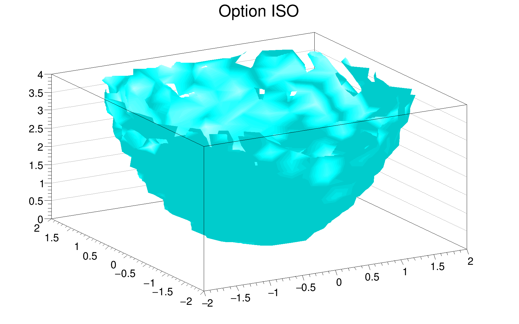
| "ISO" | Draw a Gouraud shaded 3d iso surface through a 3d histogram. It paints one surface at the value computed as follow: SumOfWeights/(NbinsX*NbinsY*NbinsZ). |
| "BOX" | Draw a for each cell with volume proportional to the content's absolute value. An hidden line removal algorithm is used |
| "BOX1" | Same as BOX but an hidden surface removal algorithm is used |
| "BOX2" | The boxes' colors are picked in the current palette according to the bins' contents |
| "BOX2Z" | Same as "BOX2". In addition the color palette is also drawn. |
| "BOX3" | Same as BOX1, but the border lines of each lego-bar are not drawn. |
| "LEGO" | Same as BOX. |
THStack)| Option | Description |
|---|---|
| " " | Default, the histograms are drawn on top of each other (as lego plots for 2D histograms). |
| "NOSTACK" | Histograms in the stack are all paint in the same pad as if the option SAME had been specified. |
| "NOSTACKB" | Histograms are drawn next to each other as bar charts. |
| "PADS" | The current pad/canvas is subdivided into a number of pads equal to the number of histograms in the stack and each histogram is paint into a separate pad. |
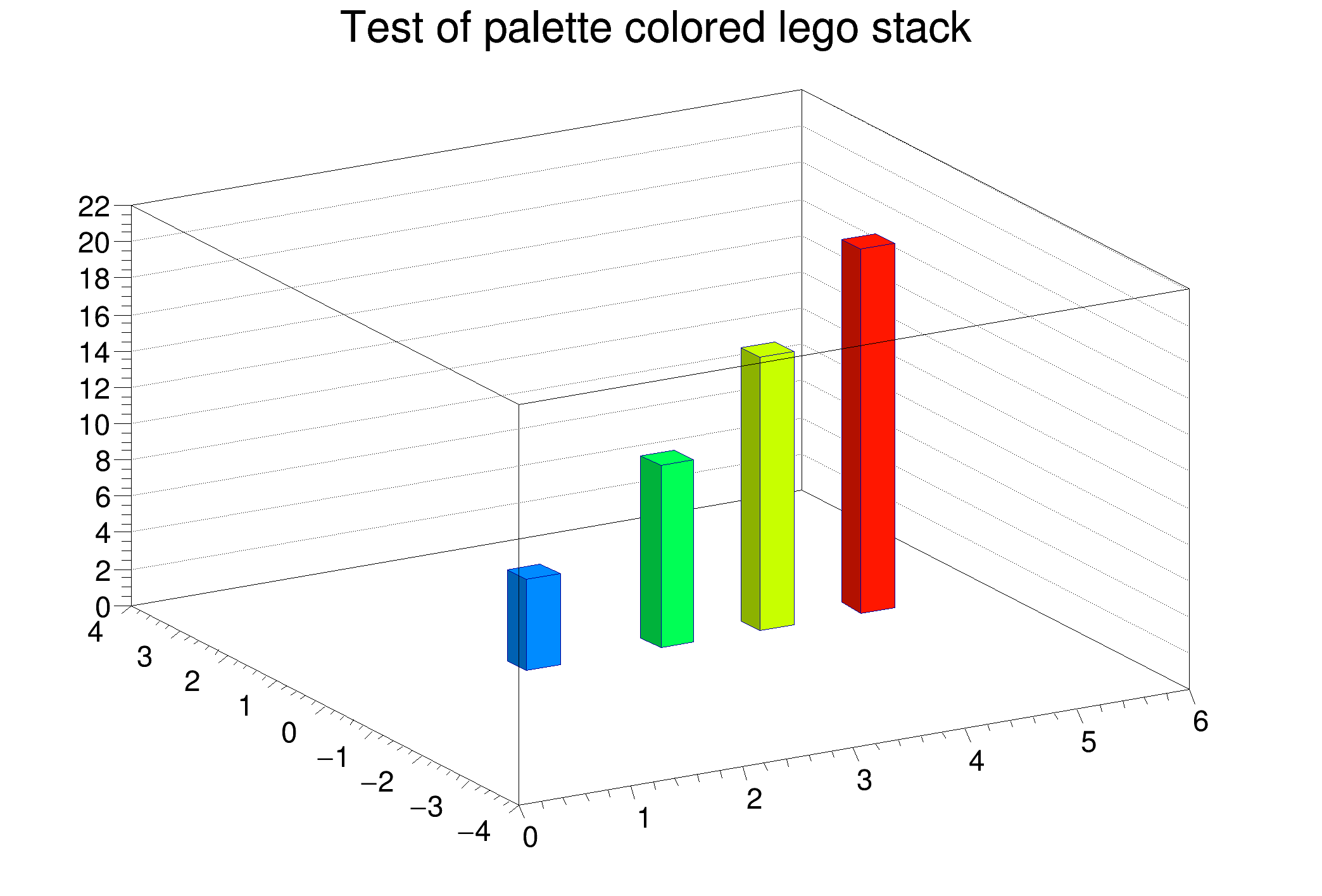
| "PFC" | Palette Fill Color: stack's fill color is taken in the current palette. |
| "PLC" | Palette Line Color: stack's line color is taken in the current palette. |
| "PMC" | Palette Marker Color: stack's marker color is taken in the current palette. |
Histograms use the current style (gStyle). When one changes the current style and would like to propagate the changes to the histogram, TH1::UseCurrentStyle should be called. Call UseCurrentStyle on each histogram is needed.
To force all the histogram to use the current style use:
gROOT->ForceStyle();
All the histograms read after this call will use the current style.
The histogram classes inherit from the attribute classes: TAttLine, TAttFill and TAttMarker. See the description of these classes for the list of options.
The TPad::SetTicks method specifies the type of tick marks on the axis. If tx = gPad->GetTickx() and ty = gPad->GetTicky() then:
tx = 1;   tick marks on top side are drawn (inside)
tx = 2;   tick marks and labels on top side are drawn
ty = 1;   tick marks on right side are drawn (inside)
ty = 2;   tick marks and labels on right side are drawn
By default only the left Y axis and X bottom axis are drawn (tx = ty = 0)
TPad::SetTicks(tx,ty) allows to set these options. See also The TAxis functions to set specific axis attributes.
In case multiple color filled histograms are drawn on the same pad, the fill area may hide the axis tick marks. One can force a redraw of the axis over all the histograms by calling:
gPad->RedrawAxis();
h->GetXaxis()->SetTitle("X axis title");
h->GetYaxis()->SetTitle("Y axis title");
The histogram title and the axis titles can be any TLatex string. The titles are part of the persistent histogram.
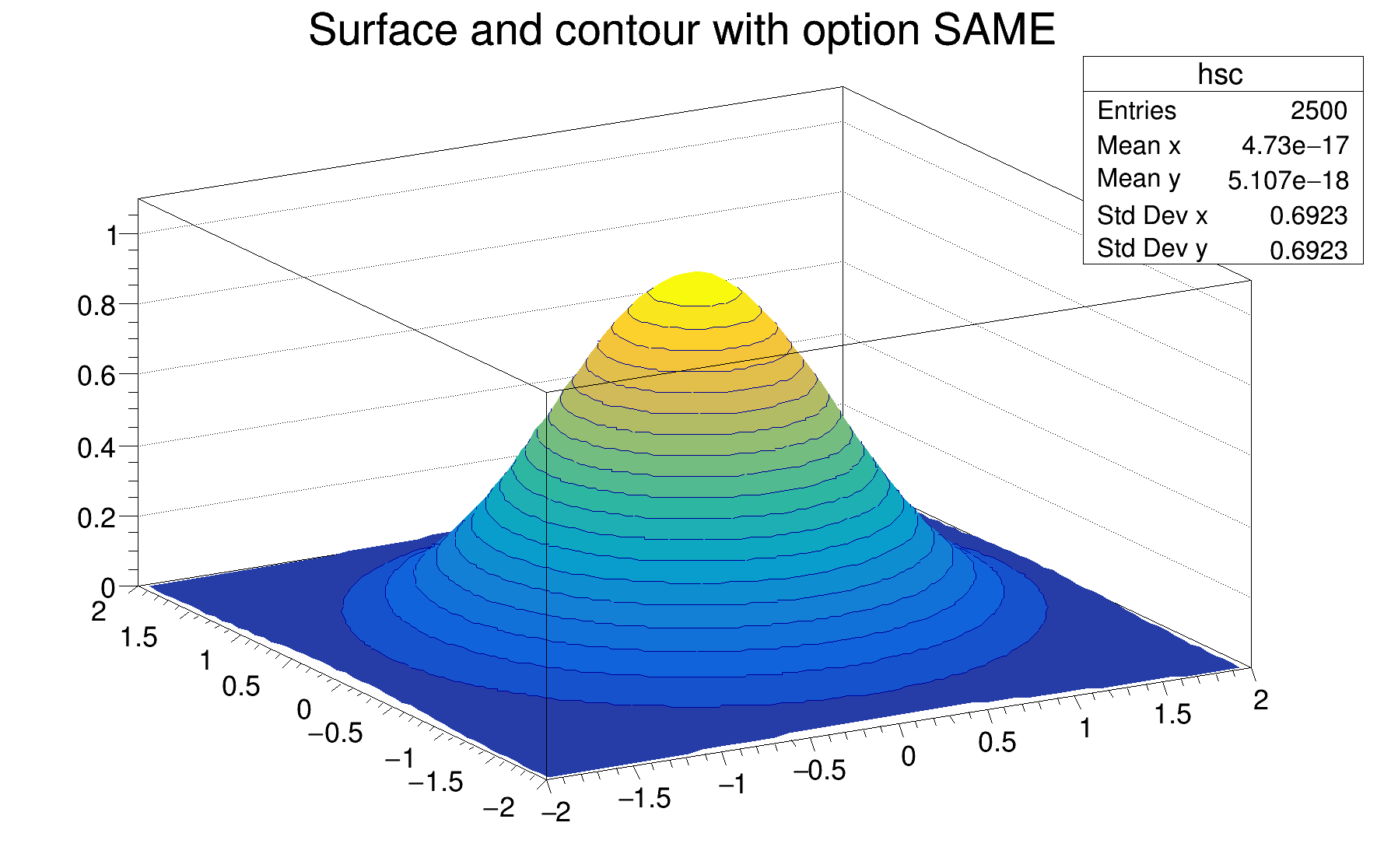
By default, when an histogram is drawn, the current pad is cleared before drawing. In order to keep the previous drawing and draw on top of it the option SAME should be use. The histogram drawn with the option SAME uses the coordinates system available in the current pad.
This option can be used alone or combined with any valid drawing option but some combinations must be use with care.
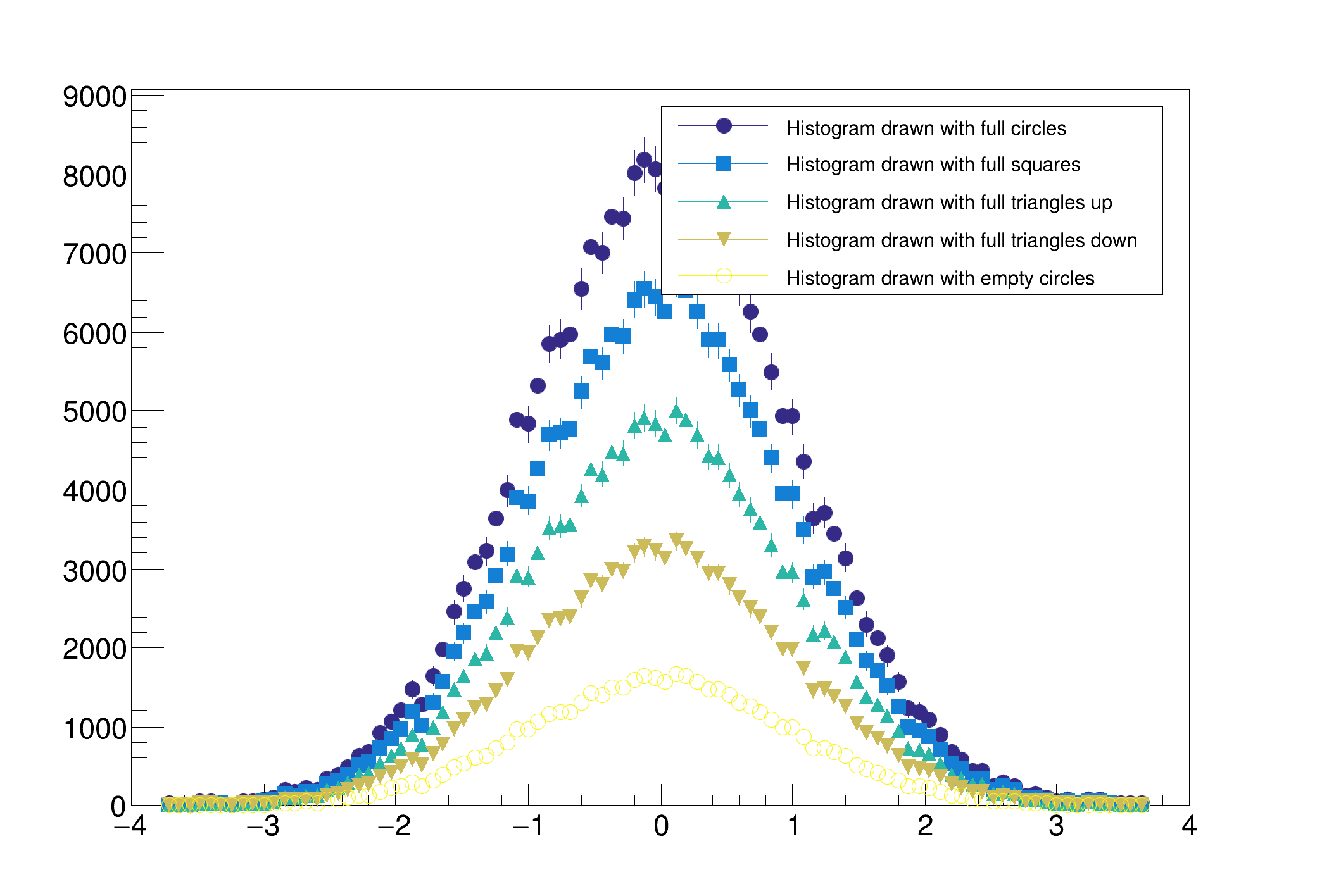
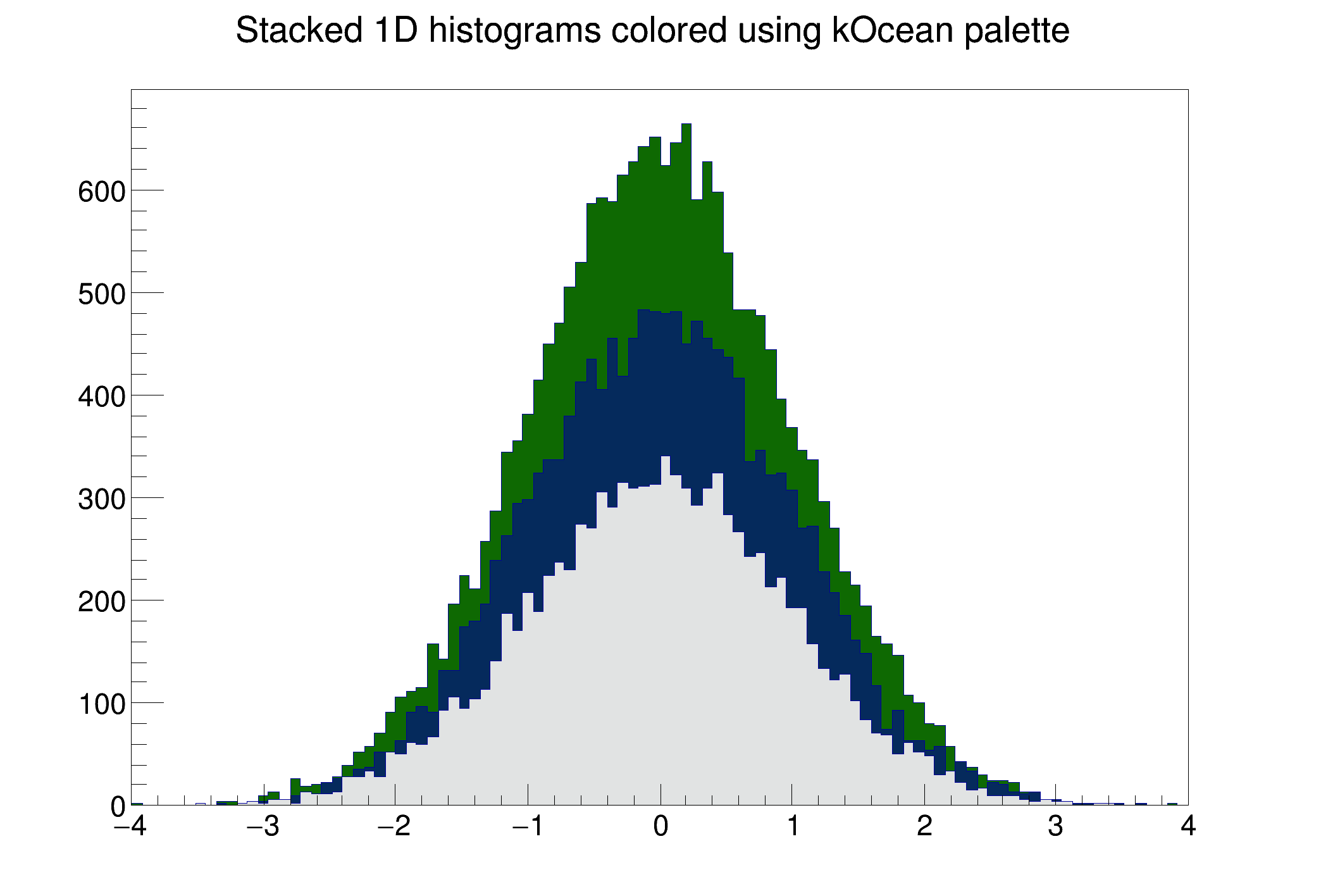
LEGO and SURF options unless the histogram plotted with the option SAME has exactly the same ranges on the X, Y and Z axis as the currently drawn histogram. To superimpose lego plots histograms' stacks should be used.When several histograms are painted in the same canvas thanks to the option "SAME" or via a THStack it might be useful to have an easy and automatic way to choose their color. The simplest way is to pick colors in the current active color palette. Palette coloring for histogram is activated thanks to the options PFC (Palette Fill Color), PLC (Palette Line Color) and PMC (Palette Marker Color). When one of these options is given to TH1::Draw the histogram get its color from the current color palette defined by gStyle->SetPalette(…). The color is determined according to the number of objects having palette coloring in the current pad.
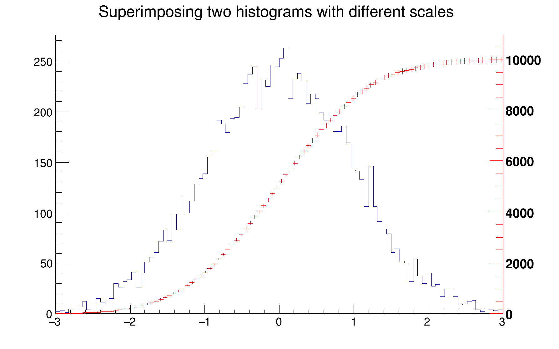
The following example creates two histograms, the second histogram is the bins integral of the first one. It shows a procedure to draw the two histograms in the same pad and it draws the scale of the second histogram using a new vertical axis on the right side. See also the tutorial transpad.C for a variant of this example.
The type of information shown in the histogram statistics box can be selected with:
gStyle->SetOptStat(mode);
The mode has up to nine digits that can be set to on (1 or 2), off (0).
mode = ksiourmen  (default = 000001111)
k = 1;  kurtosis printed
k = 2;  kurtosis and kurtosis error printed
s = 1;  skewness printed
s = 2;  skewness and skewness error printed
i = 1;  integral of bins printed
i = 2;  integral of bins with option "width" printed
o = 1;  number of overflows printed
u = 1;  number of underflows printed
r = 1;  standard deviation printed
r = 2;  standard deviation and standard deviation error printed
m = 1;  mean value printed
m = 2;  mean and mean error values printed
e = 1;  number of entries printed
n = 1;  name of histogram is printed
For example:
gStyle->SetOptStat(11);
displays only the name of histogram and the number of entries, whereas:
gStyle->SetOptStat(1101);
displays the name of histogram, mean value and standard deviation.
WARNING 1: never do:
gStyle->SetOptStat(0001111);
but instead do:
gStyle->SetOptStat(1111);
because 0001111 will be taken as an octal number!
WARNING 2: for backward compatibility with older versions
gStyle->SetOptStat(1);
is taken as:
gStyle->SetOptStat(1111)
To print only the name of the histogram do:
gStyle->SetOptStat(1000000001);
NOTE that in case of 2D histograms, when selecting only underflow (10000) or overflow (100000), the statistics box will show all combinations of underflow/overflows and not just one single number.
The parameter mode can be any combination of the letters kKsSiIourRmMen
k :  kurtosis printed
K :  kurtosis and kurtosis error printed
s :  skewness printed
S :  skewness and skewness error printed
i :  integral of bins printed
I :  integral of bins with option "width" printed
o :  number of overflows printed
u :  number of underflows printed
r :  standard deviation printed
R :  standard deviation and standard deviation error printed
m :  mean value printed
M :  mean value mean error values printed
e :  number of entries printed
n :  name of histogram is printed
For example, to print only name of histogram and number of entries do:
gStyle->SetOptStat("ne");
To print only the name of the histogram do:
gStyle->SetOptStat("n");
The default value is:
gStyle->SetOptStat("nemr");
When a histogram is painted, a TPaveStats object is created and added to the list of functions of the histogram. If a TPaveStats object already exists in the histogram list of functions, the existing object is just updated with the current histogram parameters.
Once a histogram is painted, the statistics box can be accessed using h->FindObject("stats"). In the command line it is enough to do:
Root > h->Draw()
Root > TPaveStats *st = (TPaveStats*)h->FindObject("stats")
because after h->Draw() the histogram is automatically painted. But in a script file the painting should be forced using gPad->Update() in order to make sure the statistics box is created:
h->Draw();
gPad->Update();
TPaveStats *st = (TPaveStats*)h->FindObject("stats");
Without gPad->Update() the line h->FindObject("stats") returns a null pointer.
When a histogram is drawn with the option SAME, the statistics box is not drawn. To force the statistics box drawing with the option SAME, the option SAMES must be used. If the new statistics box hides the previous statistics box, one can change its position with these lines (h being the pointer to the histogram):
Root > TPaveStats *st = (TPaveStats*)h->FindObject("stats")
Root > st->SetX1NDC(newx1); //new x start position
Root > st->SetX2NDC(newx2); //new x end position
To change the type of information for an histogram with an existing TPaveStats one should do:
st->SetOptStat(mode);
Where mode has the same meaning than when calling gStyle->SetOptStat(mode) (see above).
One can delete the statistics box for a histogram TH1* h with:
h->SetStats(0)
and activate it again with:
h->SetStats(1).
Labels used in the statistics box ("Mean", "Std Dev", ...) can be changed from $ROOTSYS/etc/system.rootrc or .rootrc (look for the string Hist.Stats.).
The type of information about fit parameters printed in the histogram statistics box can be selected via the parameter mode. The parameter mode can be = pcev (default = 0111)
p = 1;  print Probability
c = 1;  print Chisquare/Number of degrees of freedom
e = 1;  print errors (if e=1, v must be 1)
v = 1;  print name/values of parameters
Example:
gStyle->SetOptFit(1011);
print fit probability, parameter names/values and errors.
v" = 1</tt> is specified, only the non-fixed parameters are shown.
2. When <tt>v" = 2
all parameters are shown.Note: gStyle->SetOptFit(1) means "default value", so it is equivalent to gStyle->SetOptFit(111)
| Option | Description |
|---|---|
| "E" | Default. Shows only the error bars, not a marker. |
| "E1" | Small lines are drawn at the end of the error bars. |
| "E2" | Error rectangles are drawn. |
| "E3" | A filled area is drawn through the end points of the vertical error bars. |
| "E4" | A smoothed filled area is drawn through the end points of the vertical error bars. |
| "E0" | Draw also bins with null contents. |
The options "E3" and "E4" draw an error band through the end points of the vertical error bars. With "E4" the error band is smoothed. Because of the smoothing algorithm used some artefacts may appear at the end of the band like in the following example. In such cases "E3" should be used instead of "E4".
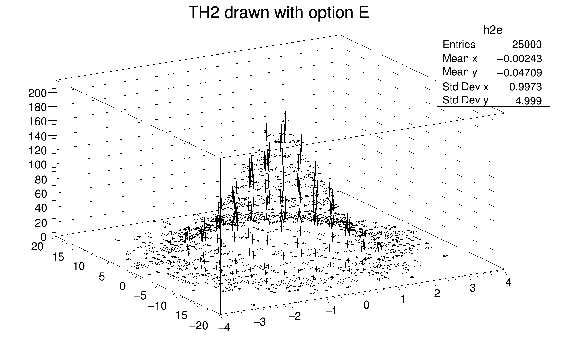
2D histograms can be drawn with error bars as shown is the following example:
The option "B" allows to draw simple vertical bar charts. The bar width is controlled with TH1::SetBarWidth(), and the bar offset within the bin, with TH1::SetBarOffset(). These two settings are useful to draw several histograms on the same plot as shown in the following example:
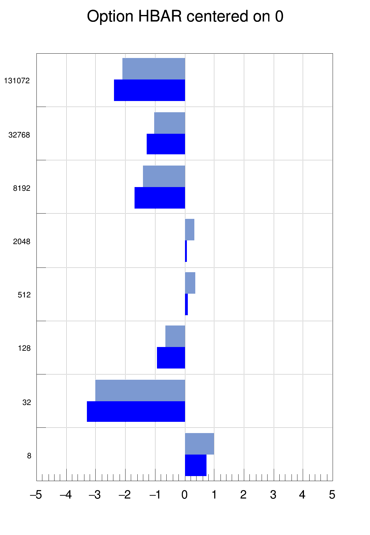
When the option bar or hbar is specified, a bar chart is drawn. A vertical bar-chart is drawn with the options bar, bar0, bar1, bar2, bar3, bar4. An horizontal bar-chart is drawn with the options hbar, hbar0, hbar1, hbar2, hbar3, hbar4 (hbars.C).
When an histogram has errors the option "HIST" together with the (h)bar option.
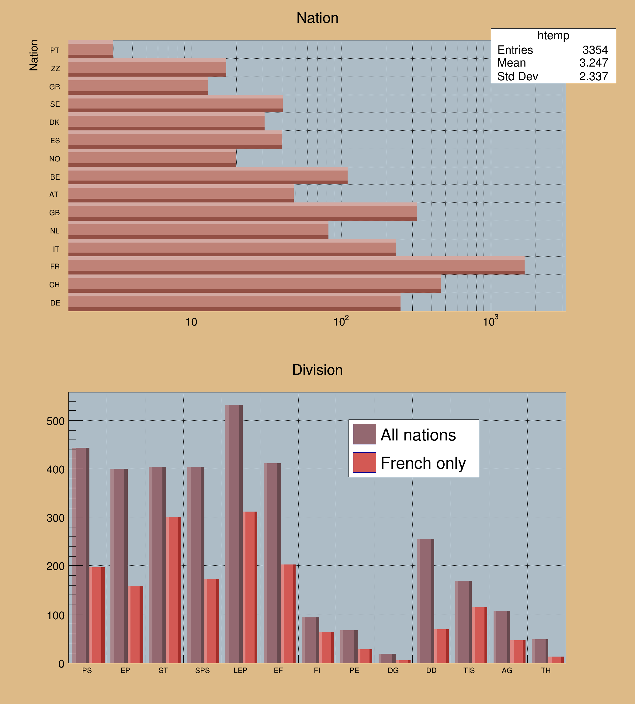
To control the bar width (default is the bin width) TH1::SetBarWidth() should be used.
To control the bar offset (default is 0) TH1::SetBarOffset() should be used.
These two parameters are useful when several histograms are plotted using the option SAME. They allow to plot the histograms next to each other.
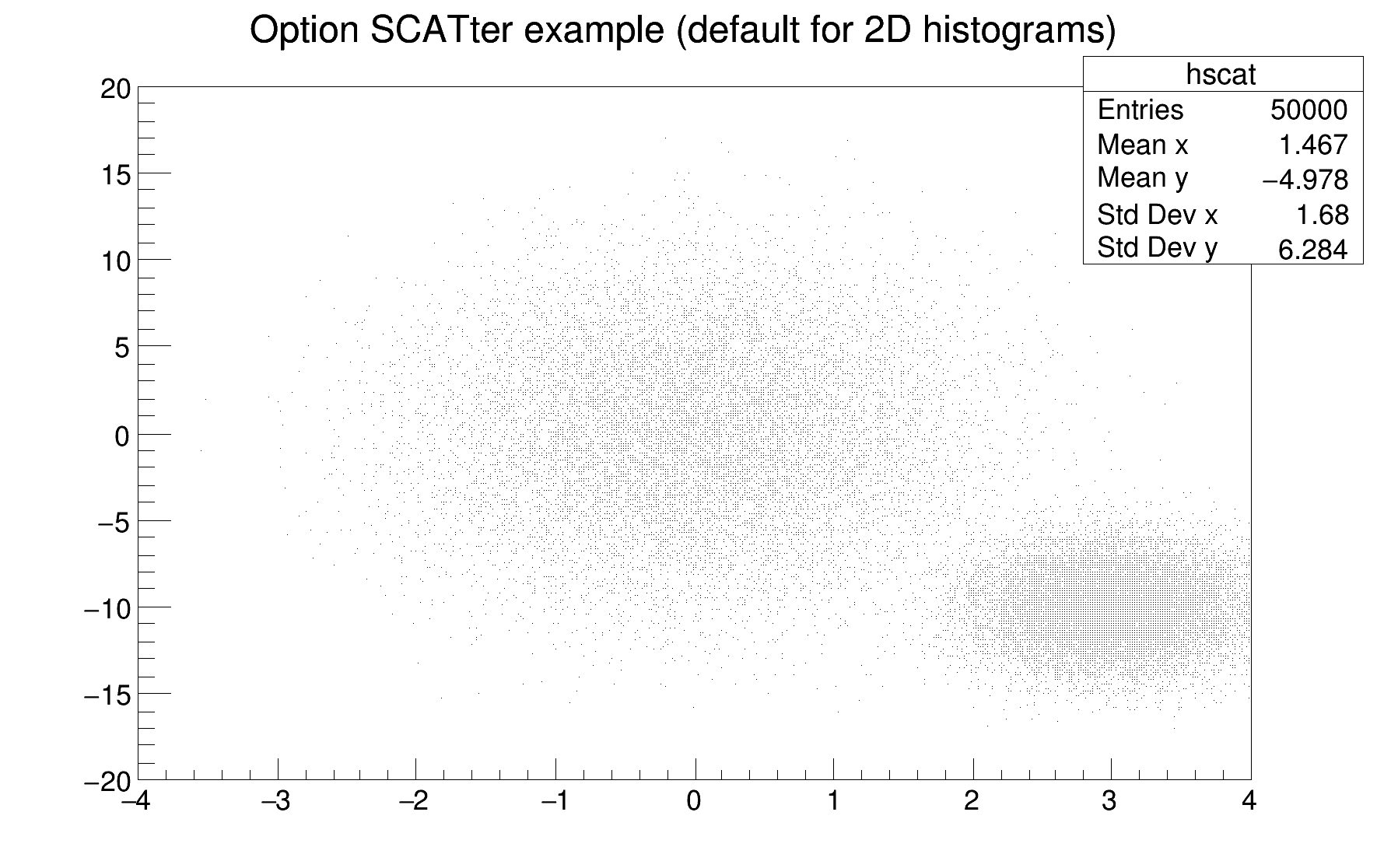
For each cell (i,j) a number of points proportional to the cell content is drawn. A maximum of kNMAX points per cell is drawn. If the maximum is above kNMAX contents are normalized to kNMAX (kNMAX=2000). If option is of the form scat=ff, (eg scat=1.8, scat=1e-3), then ff is used as a scale factor to compute the number of dots. scat=1 is the default.
By default the scatter plot is painted with a "dot marker" which not scalable (see the TAttMarker documentation). To change the marker size, a scalable marker type should be used. For instance a circle (marker style 20).
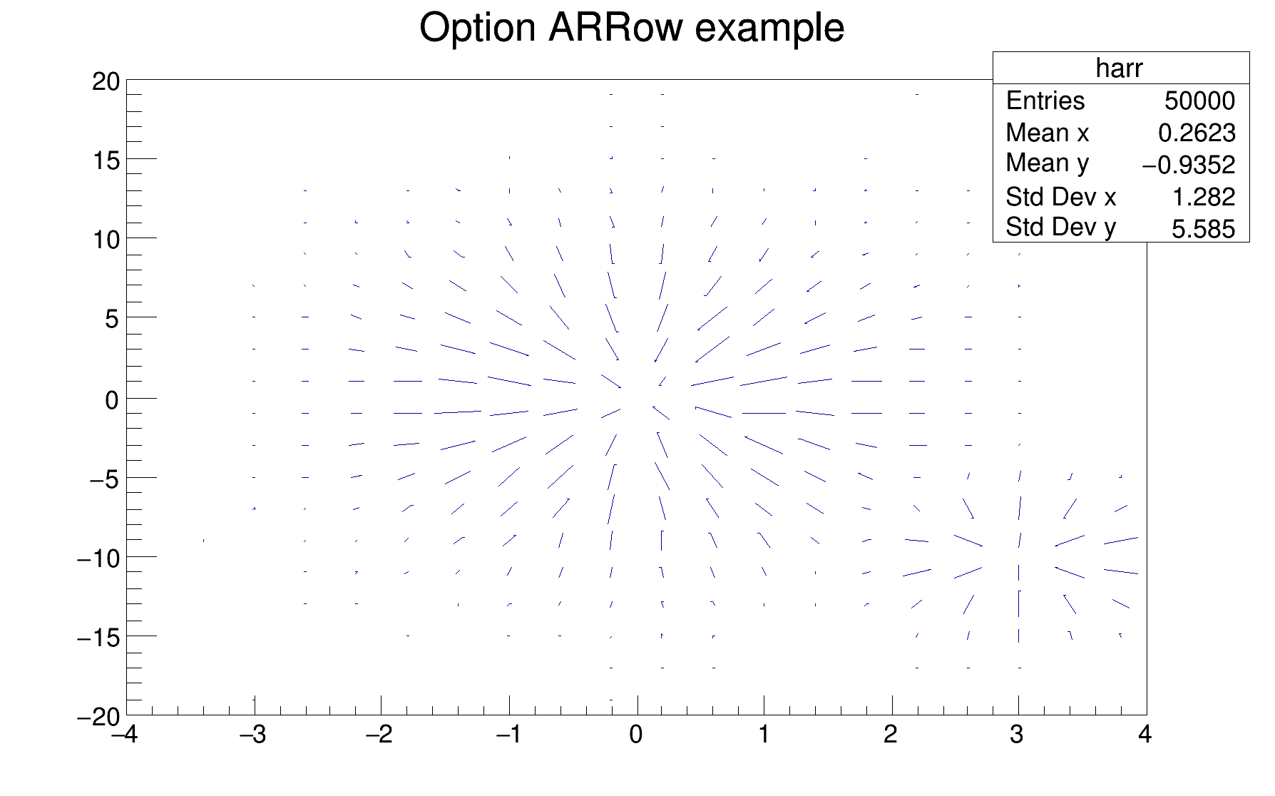
Shows gradient between adjacent cells. For each cell (i,j) an arrow is drawn The orientation of the arrow follows the cell gradient.
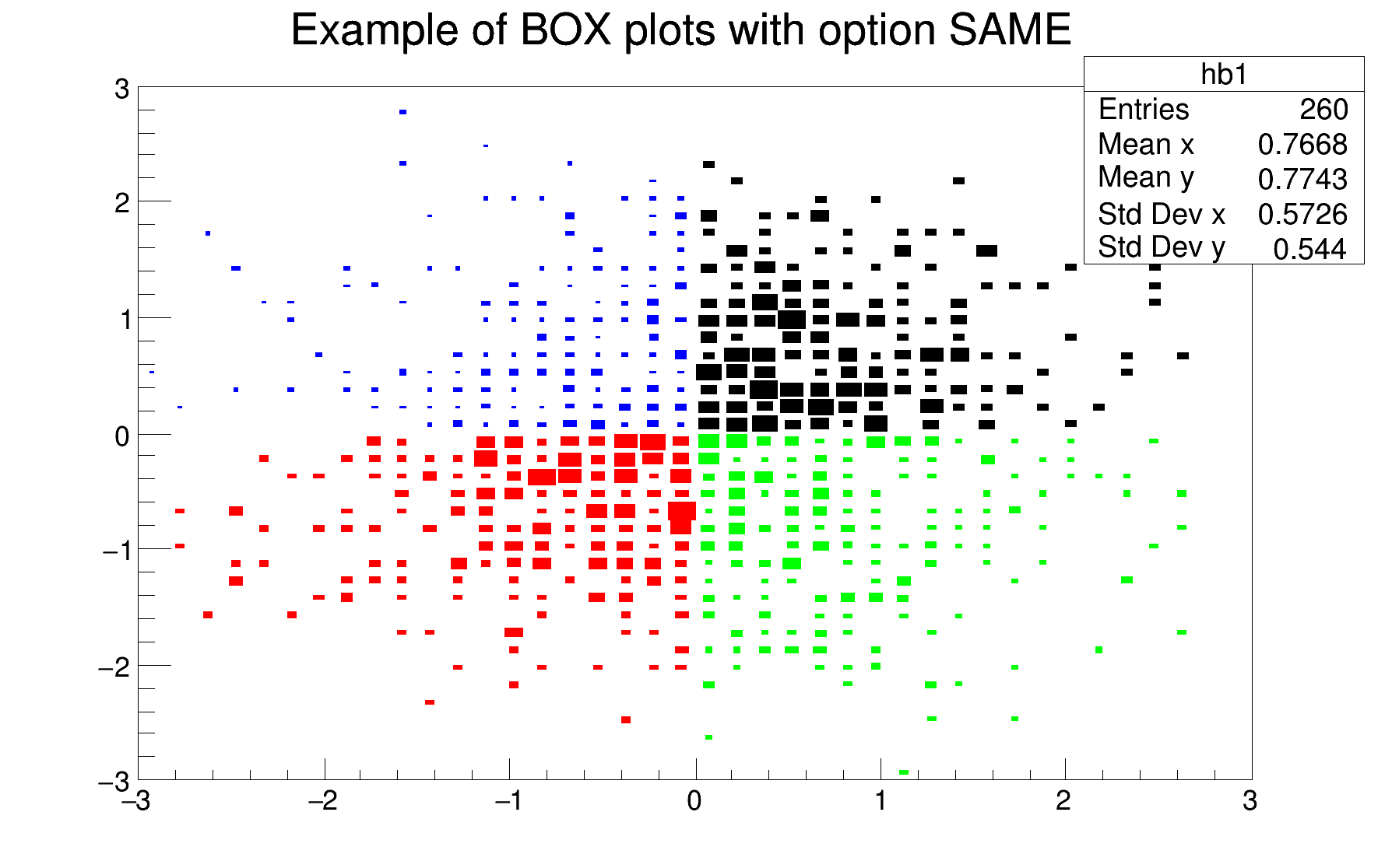
For each cell (i,j) a box is drawn. The size (surface) of the box is proportional to the absolute value of the cell content. The cells with a negative content are drawn with a X on top of the box.
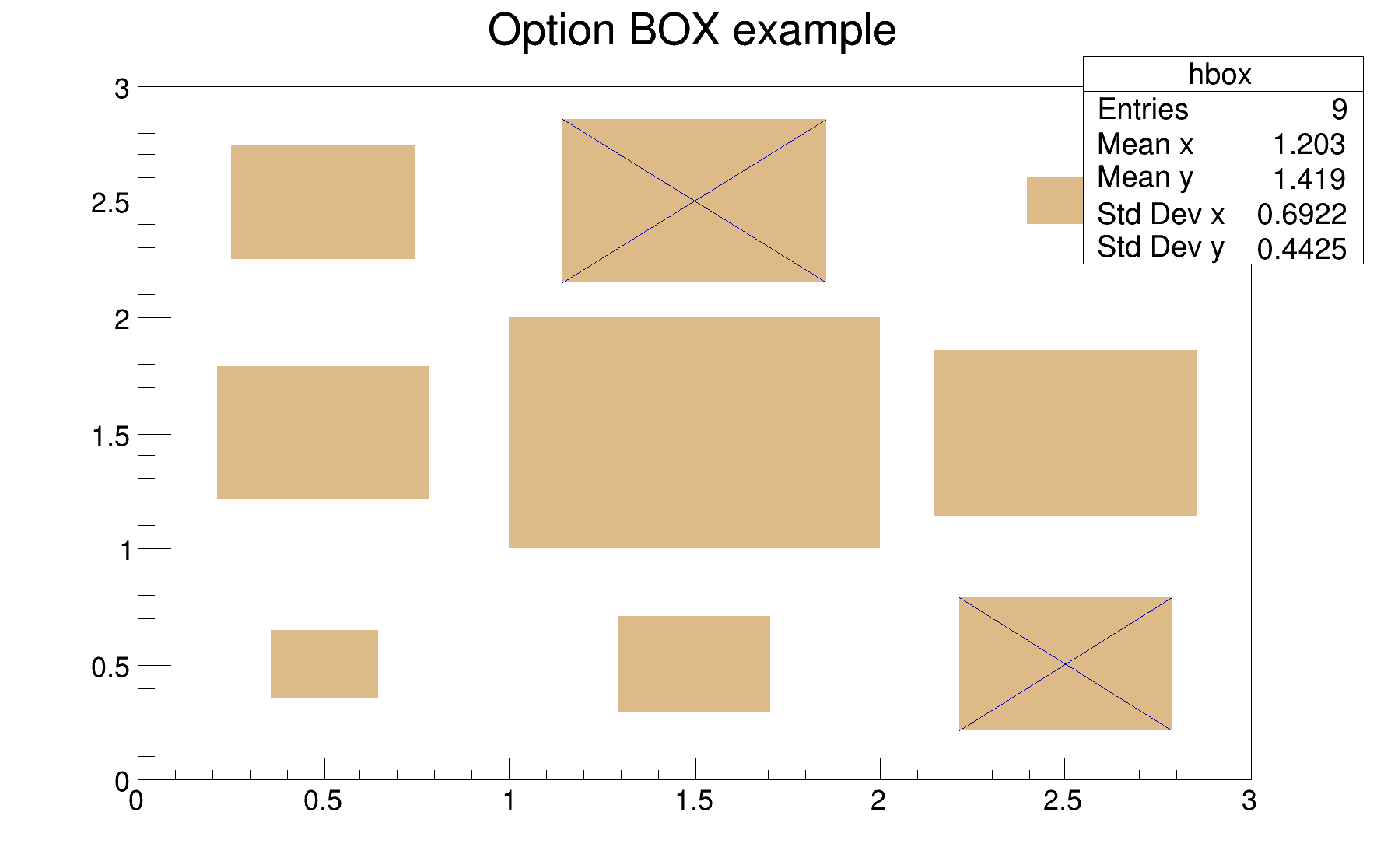
With option BOX1 a button is drawn for each cell with surface proportional to content's absolute value. A sunken button is drawn for negative values a raised one for positive.
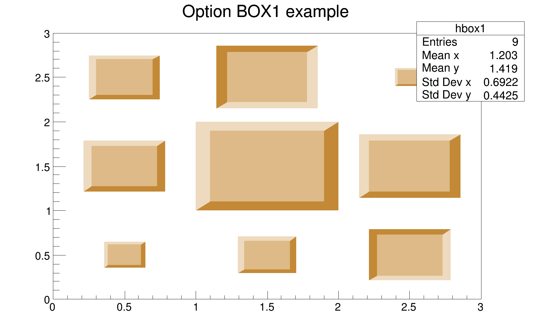
When the option SAME (or "SAMES") is used with the option BOX, the boxes' sizes are computing taking the previous plots into account. The range along the Z axis is imposed by the first plot (the one without option SAME); therefore the order in which the plots are done is relevant.
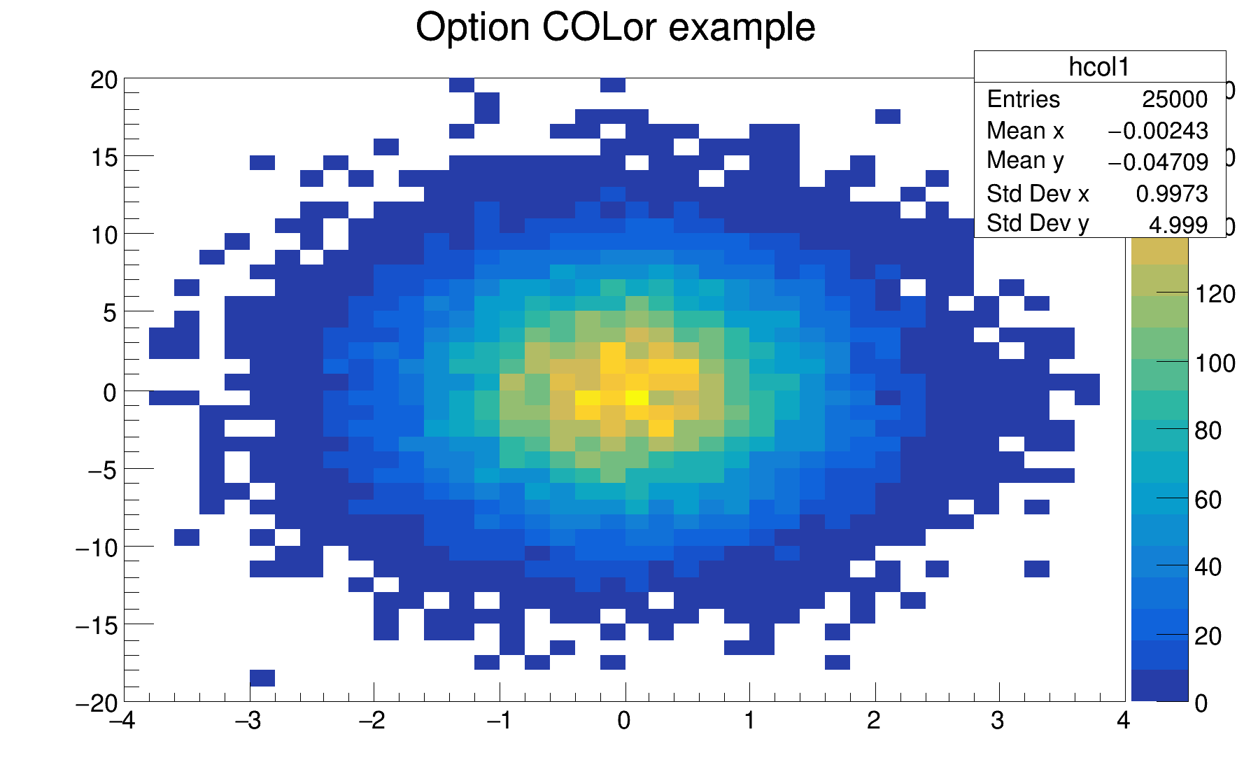
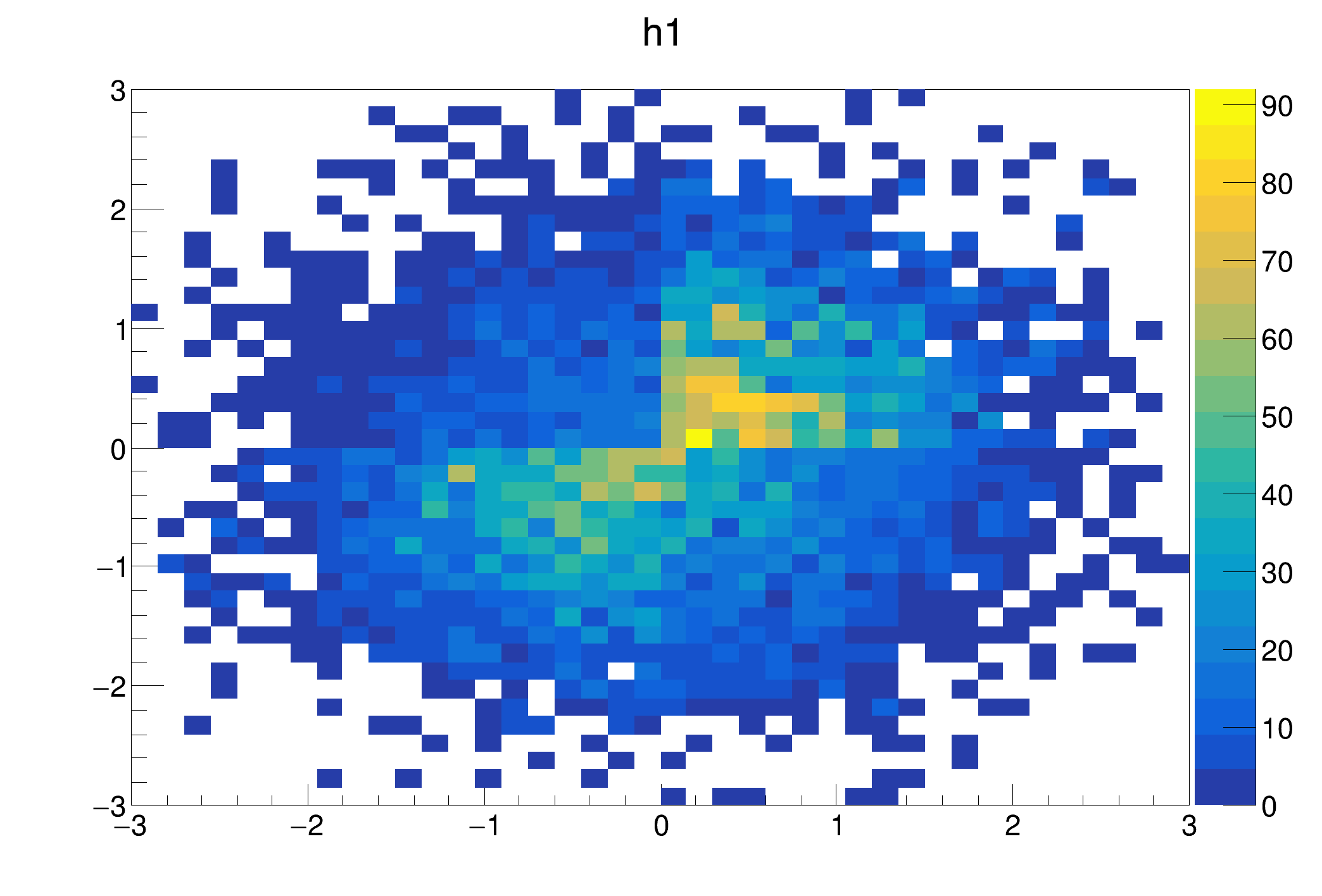
For each cell (i,j) a box is drawn with a color proportional to the cell content.
The color table used is defined in the current style.
If the histogram's minimum and maximum are the same (flat histogram), the mapping on colors is not possible, therefore nothing is painted. To paint a flat histogram it is enough to set the histogram minimum (TH1::SetMinimum()) different from the bins' content.
The default number of color levels used to paint the cells is 20. It can be changed with TH1::SetContour() or TStyle::SetNumberContours(). The higher this number is, the smoother is the color change between cells.
The color palette in TStyle can be modified via gStyle->SetPalette().
All the non-empty bins are painted. Empty bins are not painted unless some bins have a negative content because in that case the null bins might be not empty.
TProfile2D histograms are handled differently because, for this type of 2D histograms, it is possible to know if an empty bin has been filled or not. So even if all the bins' contents are positive some empty bins might be painted. And vice versa, if some bins have a negative content some empty bins might be not painted.
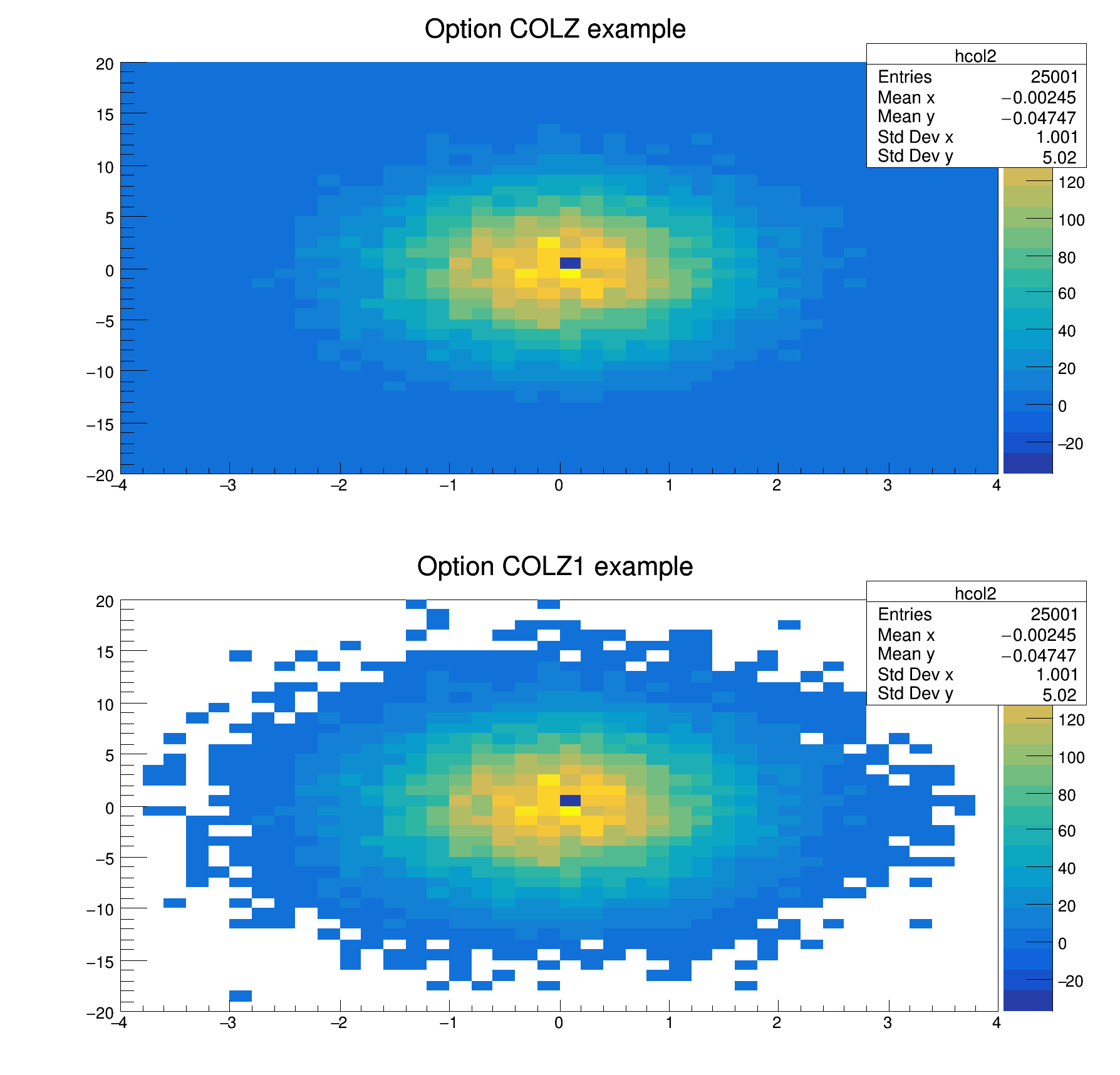
Combined with the option COL, the option Z allows to display the color palette defined by gStyle->SetPalette().
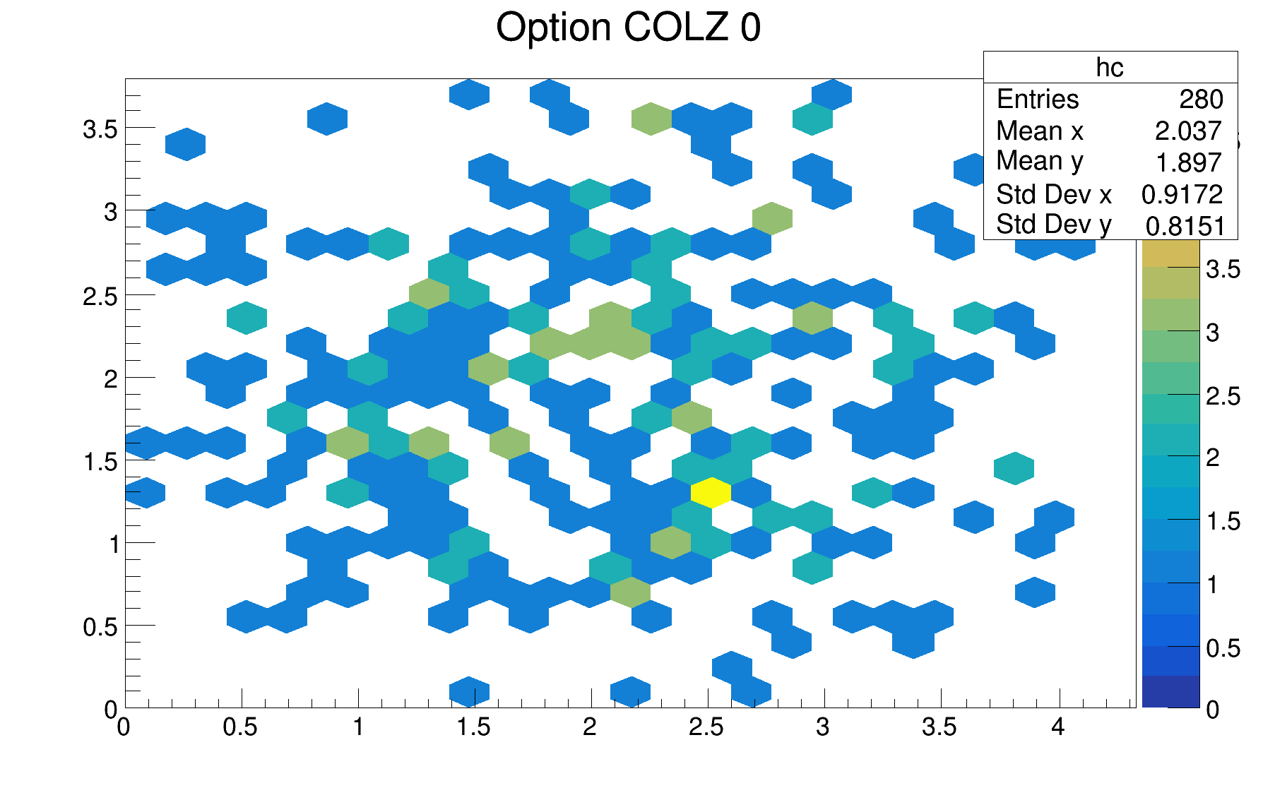
In the following example, the histogram has only positive bins; the empty bins (containing 0) are not drawn.
In the first plot of following example, the histogram has some negative bins; the empty bins (containing 0) are drawn. In some cases one wants to not draw empty bins (containing 0) of histograms having a negative minimum. The option 1, used to produce the second plot in the following picture, allows to do that.
When the maximum of the histogram is set to a smaller value than the real maximum, the bins having a content between the new maximum and the real maximum are painted with the color corresponding to the new maximum.
When the minimum of the histogram is set to a greater value than the real minimum, the bins having a value between the real minimum and the new minimum are not drawn unless the option 0 is set.
The following example illustrates the option 0 combined with the option COL.
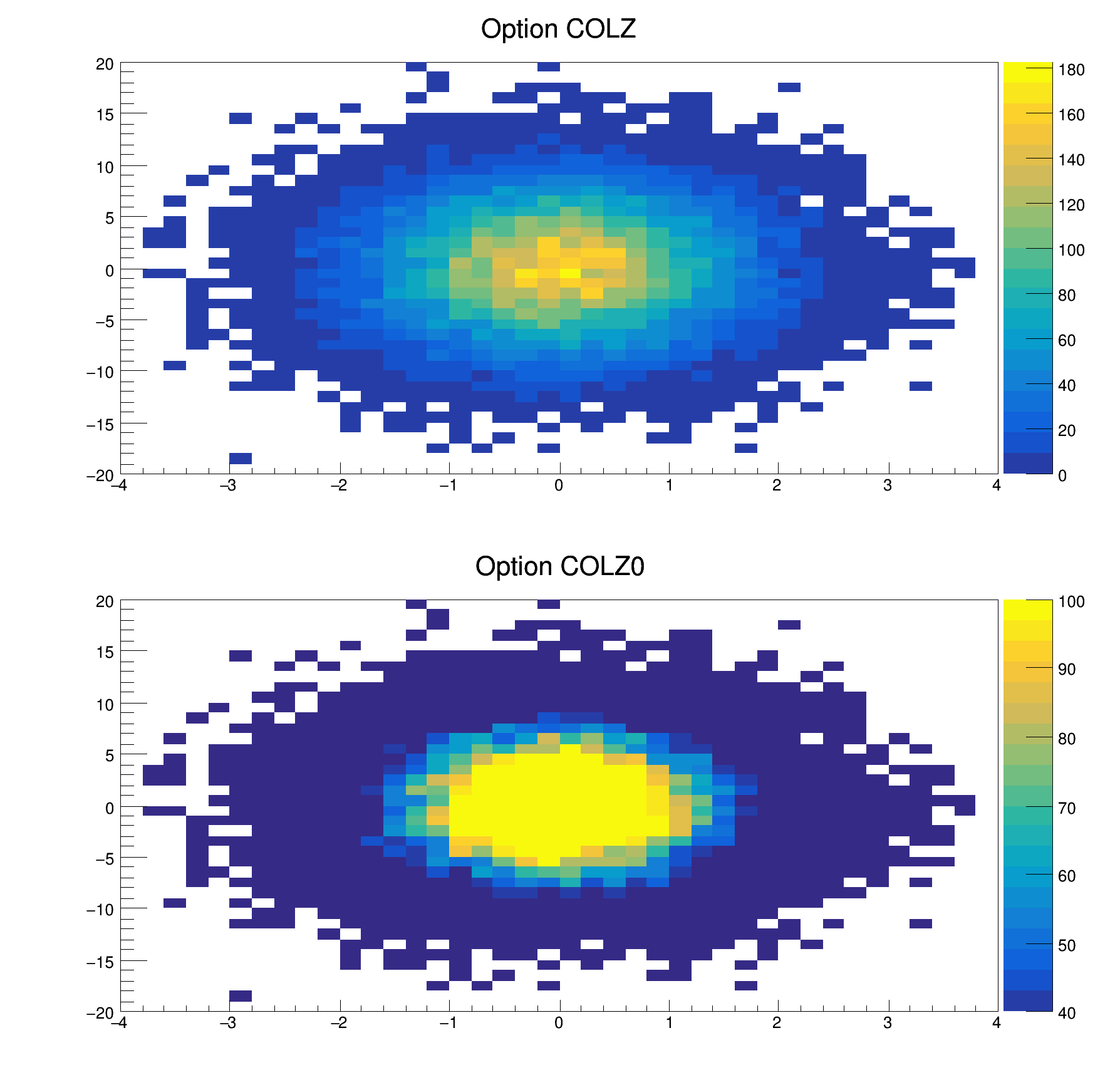
When the option SAME (or "SAMES") is used with the option COL, the boxes' color are computing taking the previous plots into account. The range along the Z axis is imposed by the first plot (the one without option SAME); therefore the order in which the plots are done is relevant.
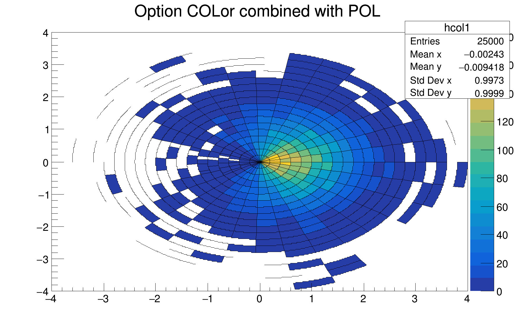
The option COL can be combined with the option POL:
A second rendering technique is also available with the COL2 and COLZ2 options.
These options provide potential performance improvements compared to the standard COL option. The performance comparison of the COL2 to the COL option depends on the histogram and the size of the rendering region in the current pad. In general, a small (approx. less than 100 bins per axis), sparsely populated TH2 will render faster with the COL option.
However, for larger histograms (approx. more than 100 bins per axis) that are not sparse, the COL2 option will provide up to 20 times performance improvements. For example, a 1000x1000 bin TH2 that is not sparse will render an order of magnitude faster with the COL2 option.
The COL2 option will also scale its performance based on the size of the pixmap the histogram image is being rendered into. It also is much better optimized for sessions where the user is forwarding X11 windows through an ssh connection.
For the most part, the COL2 and COLZ2 options are a drop in replacement to the COL and COLZ options. There is one major difference and that concerns the treatment of bins with zero content. The COL2 and COLZ2 options color these bins the color of zero.
COL2 option renders the histogram as a bitmap. Therefore it cannot be saved in vector graphics file format like PostScript or PDF (an empty image will be generated). It can be saved only in bitmap files like PNG format for instance.
The mechanism behind Candle plots and Violin plots is very similar. Because of this they are implemented in the same class TCandle. The keywords CANDLE or VIOLIN will initiate the drawing of the corresponding plots. Followed by the keyword the user can select a plot direction (X or V for vertical projections, or Y or H for horizontal projections) and/or predefined definitions (1-6 for candles, 1-2 for violins). The order doesn't matter. Default is X and 1.
Instead of using the predefined representations, the candle and violin parameters can be changed individually. In that case the option have the following form:
CANDLEX(<option-string>)
CANDLEY(<option-string>)
VIOLINX(<option-string>)
VIOLINY(<option-string>).
All zeros at the beginning of option-string can be omitted.
option-string consists eight values, defined as follow:
"CANDLEX(zhpawMmb)"
Where:
b = 0; no box drawnb = 1; the box is drawn. As the candle-plot is also called a box-plot it makes sense in the very most cases to always draw the boxb = 2; draw a filled box with borderm = 0; no median drawnm = 1; median is drawn as a linem = 2; median is drawn with errors (notches)m = 3; median is drawn as a circleM = 0; no mean drawnM = 1; mean is drawn as a dashed lineM = 3; mean is drawn as a circlew = 0; no whisker drawnw = 1; whisker is drawn to end of distribution.w = 2; whisker is drawn to max 1.5*iqra = 0; no anchor drawna = 1; the anchors are drawnp = 0; no points drawnp = 1; only outliers are drawnp = 2; all datapoints are drawnp = 3: all datapoints are drawn scatteredh = 0; no histogram is drawnh = 1; histogram at the left or bottom side is drawnh = 2; histogram at the right or top side is drawnh = 3; histogram at left and right or top and bottom (violin-style) is drawnz = 0; no zero indicator line is drawnz = 1; zero indicator line is drawn.As one can see all individual options for both candle and violin plots can be accessed by this mechanism. In deed the keywords CANDLE(<option-string>) and VIOLIN(<option-string>) have the same meaning. So you can parametrise an option-string for a candle plot and use the keywords VIOLIN and vice versa, if you wish.
Using a logarithmic x- or y-axis is possible for candle and violin charts.
a logarithmic z-axis is possible, too but will only affect violin charts of course.
A Candle plot (also known as a "box plot" or "whisker plot") was invented in 1977 by John Tukey. It is a convenient way to describe graphically a data distribution (D) with only five numbers:
In this implementation a TH2 is considered as a collection of TH1 along X (option CANDLE or CANDLEX) or Y (option CANDLEY). Each TH1 is represented as one candle.
The candle reduces the information coming from a whole distribution into few values. Independently from the number of entries or the significance of the underlying distribution a candle will always look like a candle. So candle plots should be used carefully in particular with unknown distributions. The definition of a candle is based on unbinned data. Here, candles are created from binned data. Because of this, the deviation is connected to the bin width used. The calculation of the quantiles normally done on unbinned data also. Because data are binned, this will only work the best possible way within the resolution of one bin
Because of all these facts one should take care that:
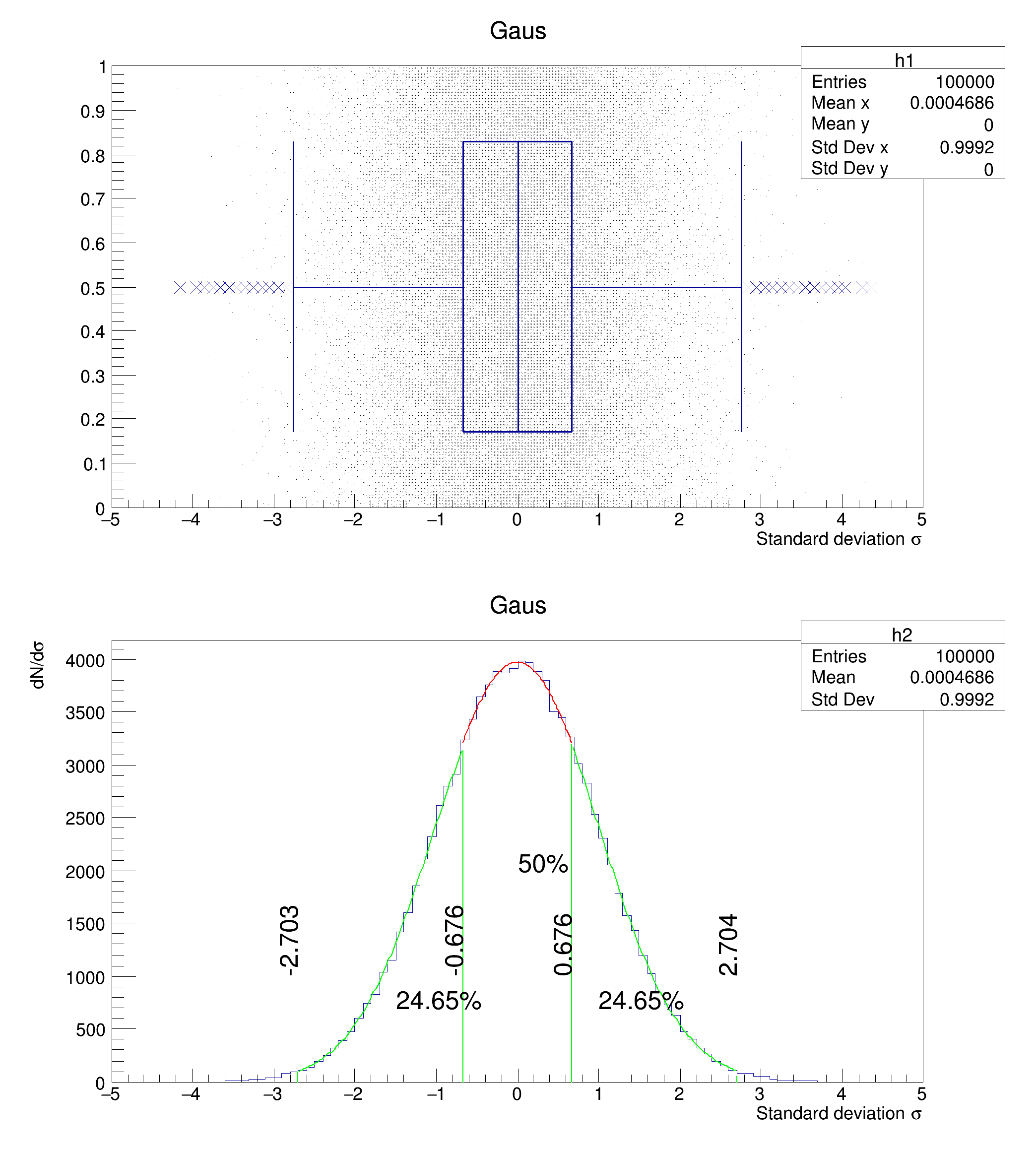
The box displays the position of the inter-quantile-range of the underlying distribution. The box contains 25% of the distribution below the median and 25% of the distribution above the median. If the underlying distribution is large enough and gaussian shaped the end-points of the box represent \( 0.6745\times\sigma \) (Where \( \sigma \) is the standard deviation of the gaussian). The width and the position of the box can be modified by SetBarWidth() and SetBarOffset(). The +-25% quantiles are calculated by the GetQuantiles() methods.
Using the static function TCandle::SetBoxRange(double) the box definition will be overwritten. E.g. using a box range of 0.68 will redefine the area of the lower box edge to the upper box edge in order to cover 68% of the distribution illustrated by that candle. The static function will affect all candle-charts in the running program. Default is 0.5.
Using the static function TCandle::SetScaledCandle(bool) the width of the box (and the whole candle) can be influenced. Deactivated, the width is constant (to be set by SetBarWidth() ). Activated, the width of the boxes will be scaled to each other based on the amount of data in the corresponding candle, the maximum width can be influenced by SetBarWidth(). The static function will affect all candle-charts in the running program. Default is false. Scaling between multiple candle-charts (using "same" or THStack) is not supported, yet
For a sorted list of numbers, the median is the value in the middle of the list. E.g. if a sorted list is made of five numbers "1,2,3,6,7" 3 will be the median because it is in the middle of the list. If the number of entries is even the average of the two values in the middle will be used. As histograms are binned data, the situation is a bit more complex. The following example shows this:
Here the bin-width is 1.0. If the two Fill(3) are commented out, as there are currently, the example will return a calculated median of 4.5, because that's the bin center of the bin in which the value 4.0 has been dropped. If the two Fill(3) are not commented out, it will return 3.75, because the algorithm tries to evenly distribute the individual values of a bin with bin content > 0. It means the sorted list would be "3.25, 3.75, 4.5".
The consequence is a median of 3.75. This shows how important it is to use a small enough bin-width when using candle-plots on binned data. If the distribution is large enough and gaussian shaped the median will be exactly equal to the mean. The median can be shown as a line or as a circle or not shown at all.
In order to show the significance of the median notched candle plots apply a "notch" or narrowing of the box around the median. The significance is defined by \( 1.57\times\frac{iqr}{N} \) and will be represented as the size of the notch (where iqr is the size of the box and N is the number of entries of the whole distribution). Candle plots like these are usually called "notched candle plots".
In case the significance of the median is greater that the size of the box, the box will have an unnatural shape. Usually it means the chart has not enough data, or that representing this uncertainty is not useful
The mean can be drawn as a dashed line or as a circle or not drawn at all. The mean is the arithmetic average of the values in the distribution. It is calculated using GetMean(). Because histograms are binned data, the mean value can differ from a calculation on the raw-data. If the distribution is large enough and gaussian shaped the mean will be exactly the median.
The whiskers represent the part of the distribution not covered by the box. The upper 25% and the lower 25% of the distribution are located within the whiskers. Two representations are available.
Using the static function TCandle::SetWhiskerRange(double) the whisker definition w=1 will be overwritten. E.g. using a whisker-range of 0.95 and w=1 will redefine the area of the lower whisker to the upper whisker in order to cover 95% of the distribution inside that candle. The static function will affect all candle-charts in the running program. Default is 1.
If the distribution is large enough and gaussian shaped, the maximum length of the whisker will be located at \( \pm 2.698 \sigma \) (when using the 1.5*iqr-definition (w=2), where \( \sigma \) is the standard deviation (see picture above). In that case 99.3% of the total distribution will be covered by the box and the whiskers, whereas 0.7% are represented by the outliers.
The anchors have no special meaning in terms of statistical calculation. They mark the end of the whiskers and they have the width of the box. Both representation with and without anchors are common.
Depending on the configuration the points can have different meanings:
Is is possible to combine all options of candle and violin plots with each other. E.g. a box-plot with a histogram.
There are six predefined candle-plot representations:
The following picture shows how the six predefined representations look.
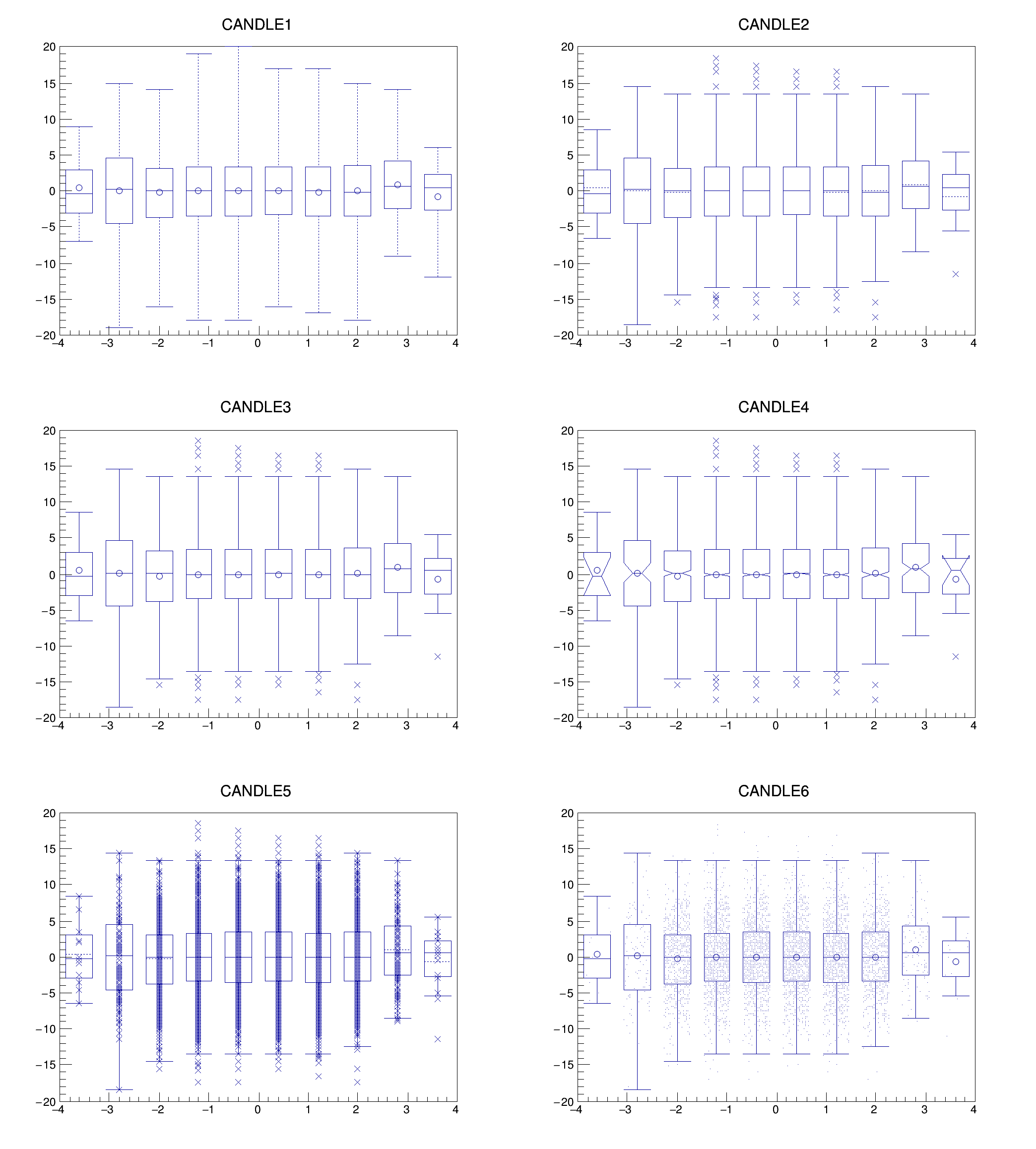
Box and improved whisker, no mean, no median, no anchor no outliers
h1->Draw("CANDLEX(2001)");
A Candle-definition like "CANDLEX2" (New standard candle with better whisker definition + outliers)
h1->Draw("CANDLEX(112111)");
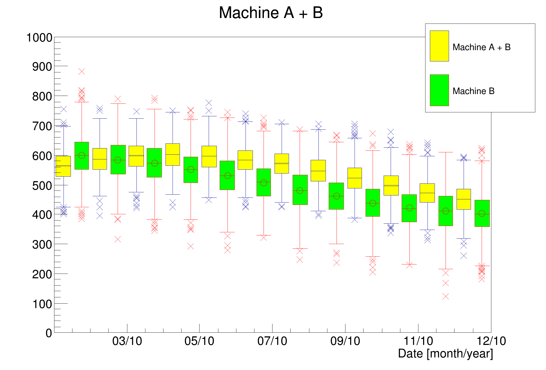
The following example shows how several candle plots can be super-imposed using the option SAME. Note that the bar-width and bar-offset are active on candle plots. Also the color, the line width, the size of the points and so on can be changed by the standard attribute setting methods such as SetLineColor() SetLineWidth().
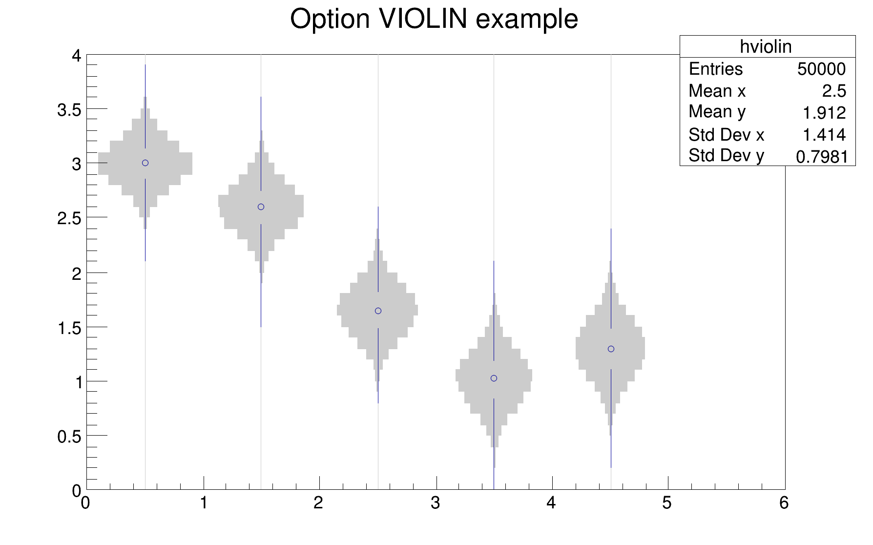
A violin plot is a candle plot that also encodes the pdf information at each point.
Quartiles and mean are also represented at each point, with a marker and two lines.
In this implementation a TH2 is considered as a collection of TH1 along X (option VIOLIN or VIOLINX) or Y (option VIOLINY).
The histogram is typically drawn to both directions with respect to the middle-line of the corresponding bin. This can be achieved by using h=3. It is possible to draw a histogram only to one side (h=1, or h=2). The maximum number of bins in the histogram is limited to 500, if the number of bins in the used histogram is higher it will be rebinned automatically. The maximum height of the histogram can be modified by using SetBarWidth() and the position can be changed with SetBarOffset(). A solid fill style is recommended.
Using the static function TCandle::SetScaledViolin(bool) the height of the histogram or the violin can be influenced. Activated, the height of the bins of the individual violins will be scaled with respect to each other, the maximum height can be influenced by SetBarWidth(). Deactivated, the height of the bin with the maximum content of each individual violin is set to a constant value using SetBarWidth(). The static function will affect all violin-charts in the running program. Default is true. Scaling between multiple violin-charts (using "same" or THStack) is not supported, yet.
Typical for violin charts is a line in the background over the whole histogram indicating the bins with zero entries. The zero indicator line can be activated with z=1. The line color will always be the same as the fill-color of the histogram.
The Mean is illustrated with the same mechanism as used for candle plots. Usually a circle is used.
The whiskers are illustrated by the same mechanism as used for candle plots. There is only one difference. When using the simple whisker definition (w=1) and the zero indicator line (z=1), then the whiskers will be forced to be solid (usually hashed)
The points are illustrated by the same mechanism as used for candle plots. E.g. VIOLIN2 uses better whisker definition (w=2) and outliers (p=1).
It is possible to combine all options of candle or violin plots with each other. E.g. a violin plot including a box-plot.
There are two predefined violin-plot representations:
A solid fill style is recommended for this plot (as opposed to a hollow or hashed style).
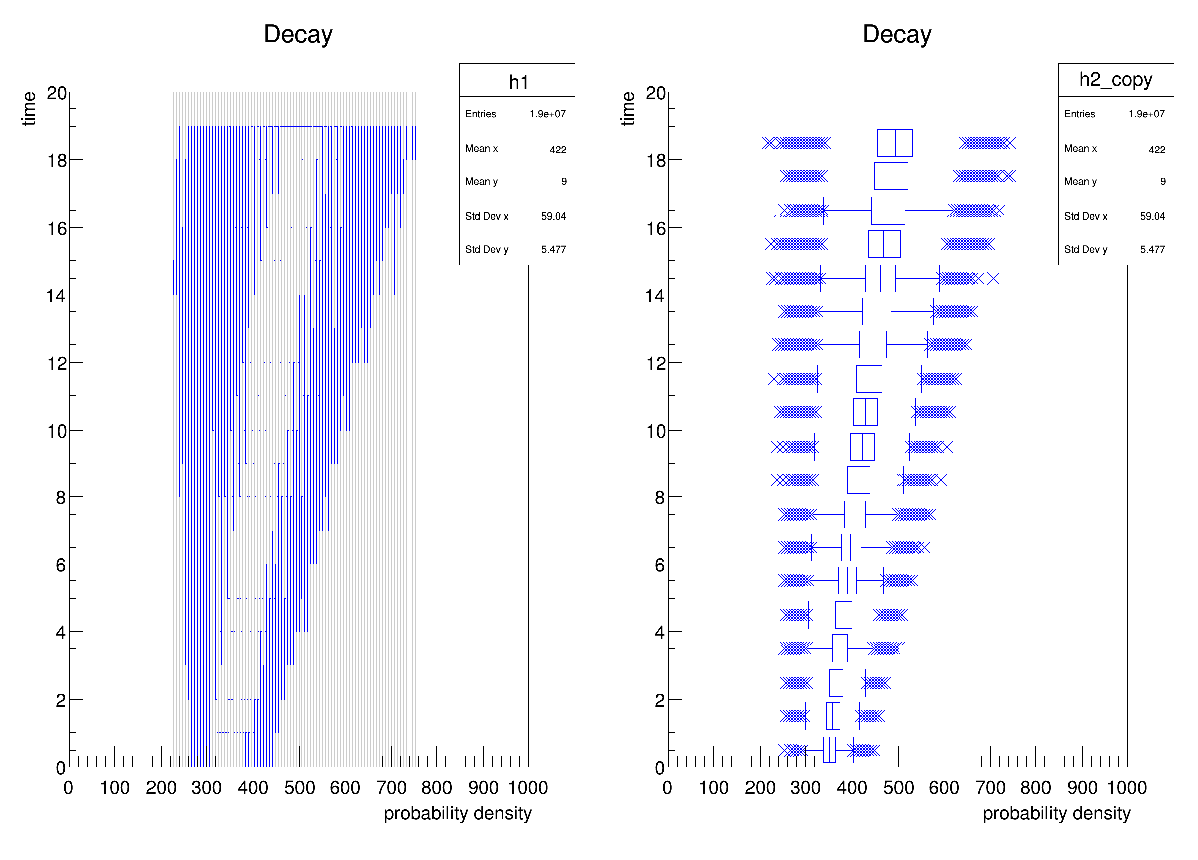
The next example illustrates a time development of a certain value:
For each bin the content is printed. The text attributes are:
gStyle->SetTextFont()).h is the histogram drawn with the option TEXT the marker size can be changed with h->SetMarkerSize(markersize)).By default the format g is used. This format can be redefined by calling gStyle->SetPaintTextFormat().
It is also possible to use TEXTnn in order to draw the text with the angle nn (0 < nn < 90).
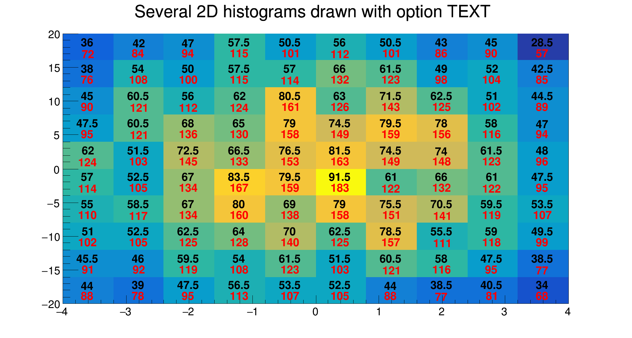
For 2D histograms the text is plotted in the center of each non empty cells. It is possible to plot empty cells by calling gStyle->SetHistMinimumZero(). For 1D histogram the text is plotted at a y position equal to the bin content.
For 2D histograms when the option "E" (errors) is combined with the option text ("TEXTE"), the error for each bin is also printed.
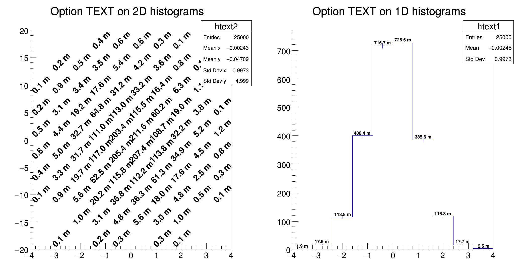
In case several histograms are drawn on top ot each other (using option SAME), the text can be shifted using SetBarOffset(). It specifies an offset for the text position in each cell, in percentage of the bin width.
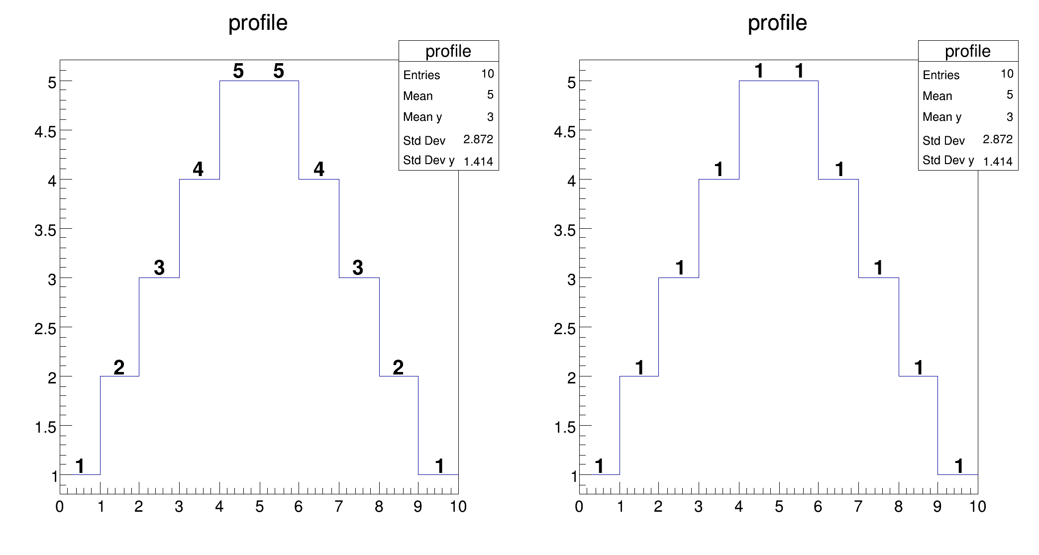
In the case of profile histograms it is possible to print the number of entries instead of the bin content. It is enough to combine the option "E" (for entries) with the option "TEXT".
The following contour options are supported:
| Option | Description |
|---|---|
| "CONT" | Draw a contour plot (same as CONT0). |
| "CONT0" | Draw a contour plot using surface colors to distinguish contours. |
| "CONT1" | Draw a contour plot using the line colors to distinguish contours. |
| "CONT2" | Draw a contour plot using the line styles to distinguish contours. |
| "CONT3" | Draw a contour plot solid lines for all contours. |
| "CONT4" | Draw a contour plot using surface colors (SURF option at theta = 0). |
| "CONT5" | Draw a contour plot using Delaunay triangles. |
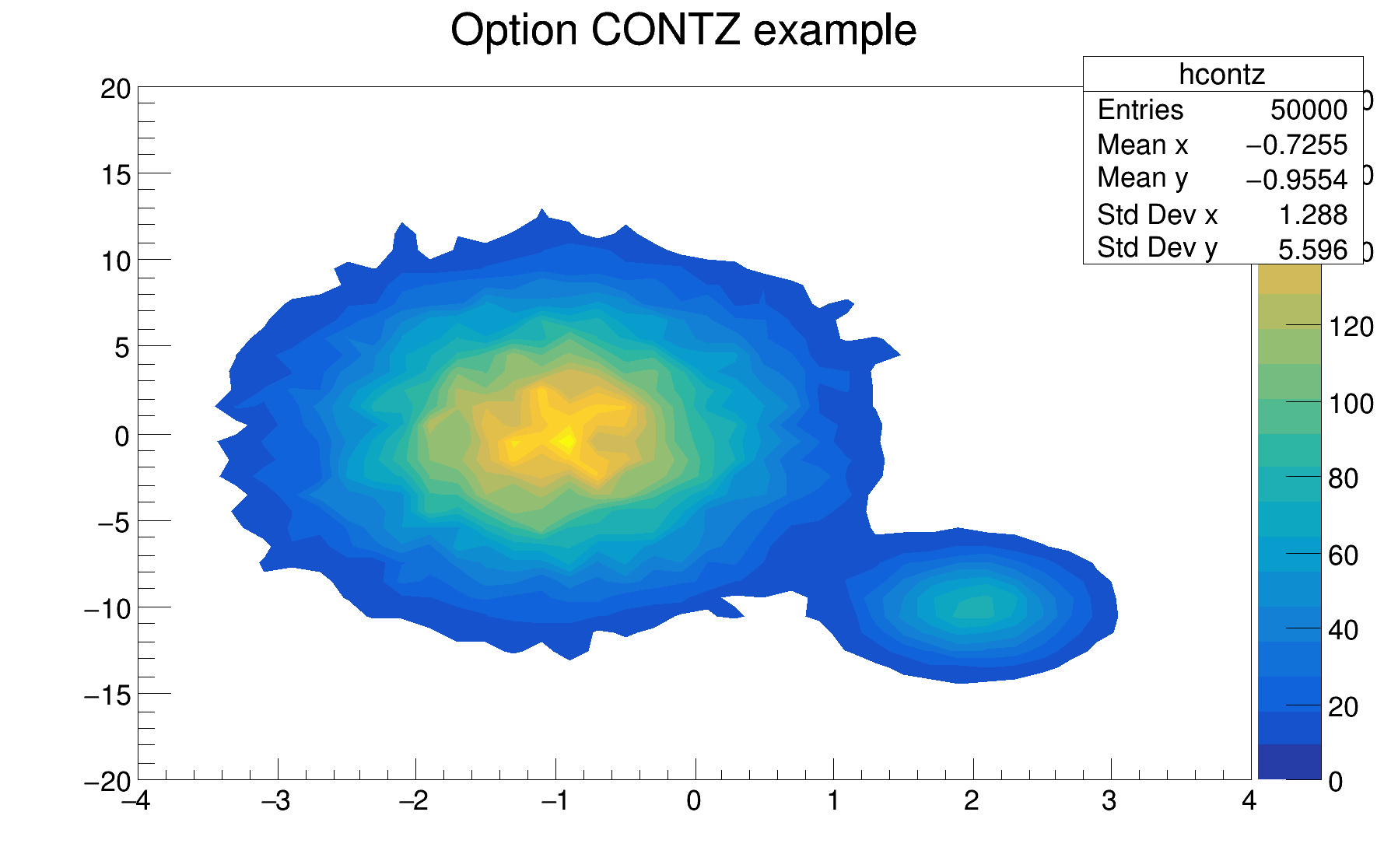
The following example shows a 2D histogram plotted with the option CONTZ. The option CONT draws a contour plot using surface colors to distinguish contours. Combined with the option CONT (or CONT0), the option Z allows to display the color palette defined by gStyle->SetPalette().
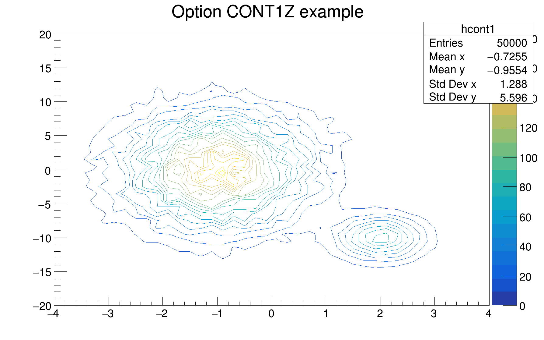
The following example shows a 2D histogram plotted with the option CONT1Z. The option CONT1 draws a contour plot using the line colors to distinguish contours. Combined with the option CONT1, the option Z allows to display the color palette defined by gStyle->SetPalette().
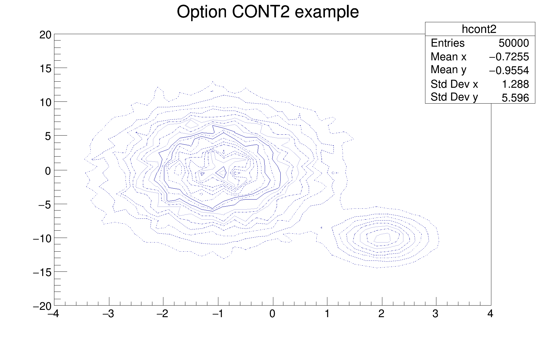
The following example shows a 2D histogram plotted with the option CONT2. The option CONT2 draws a contour plot using the line styles to distinguish contours.
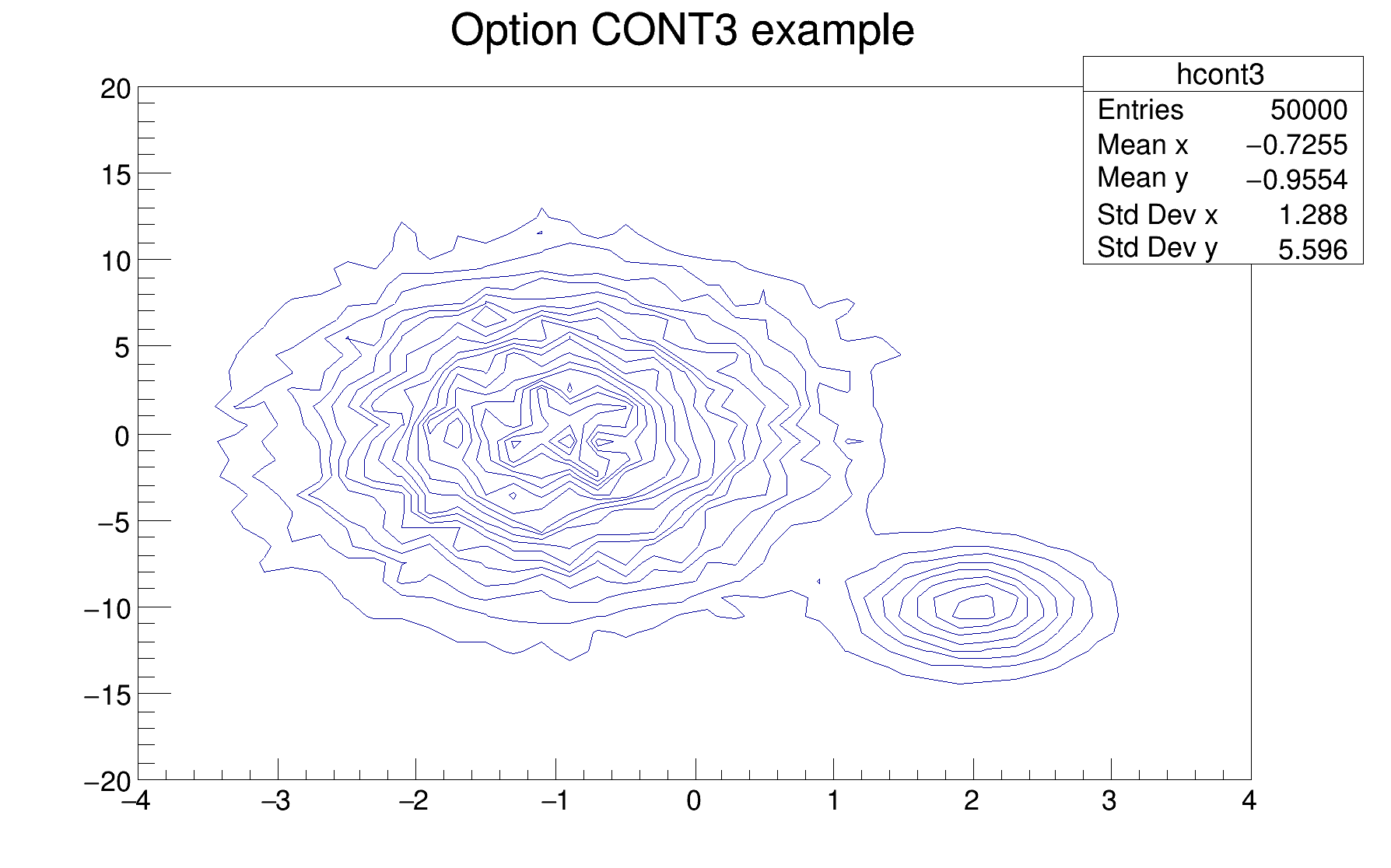
The following example shows a 2D histogram plotted with the option CONT3. The option CONT3 draws contour plot solid lines for all contours.
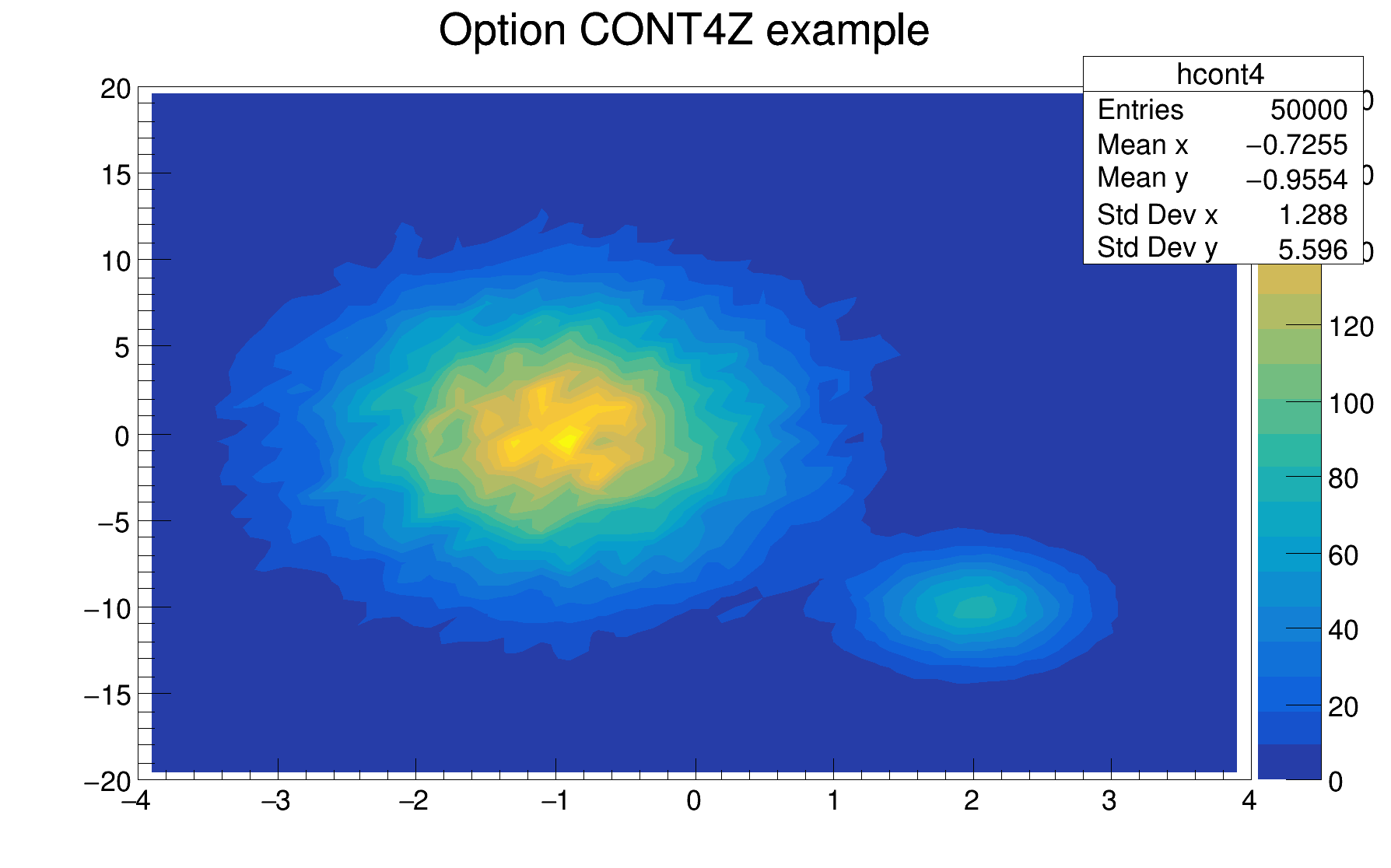
The following example shows a 2D histogram plotted with the option CONT4. The option CONT4 draws a contour plot using surface colors to distinguish contours (SURF option at theta = 0). Combined with the option CONT (or CONT0), the option Z allows to display the color palette defined by gStyle->SetPalette().
The default number of contour levels is 20 equidistant levels and can be changed with TH1::SetContour() or TStyle::SetNumberContours().
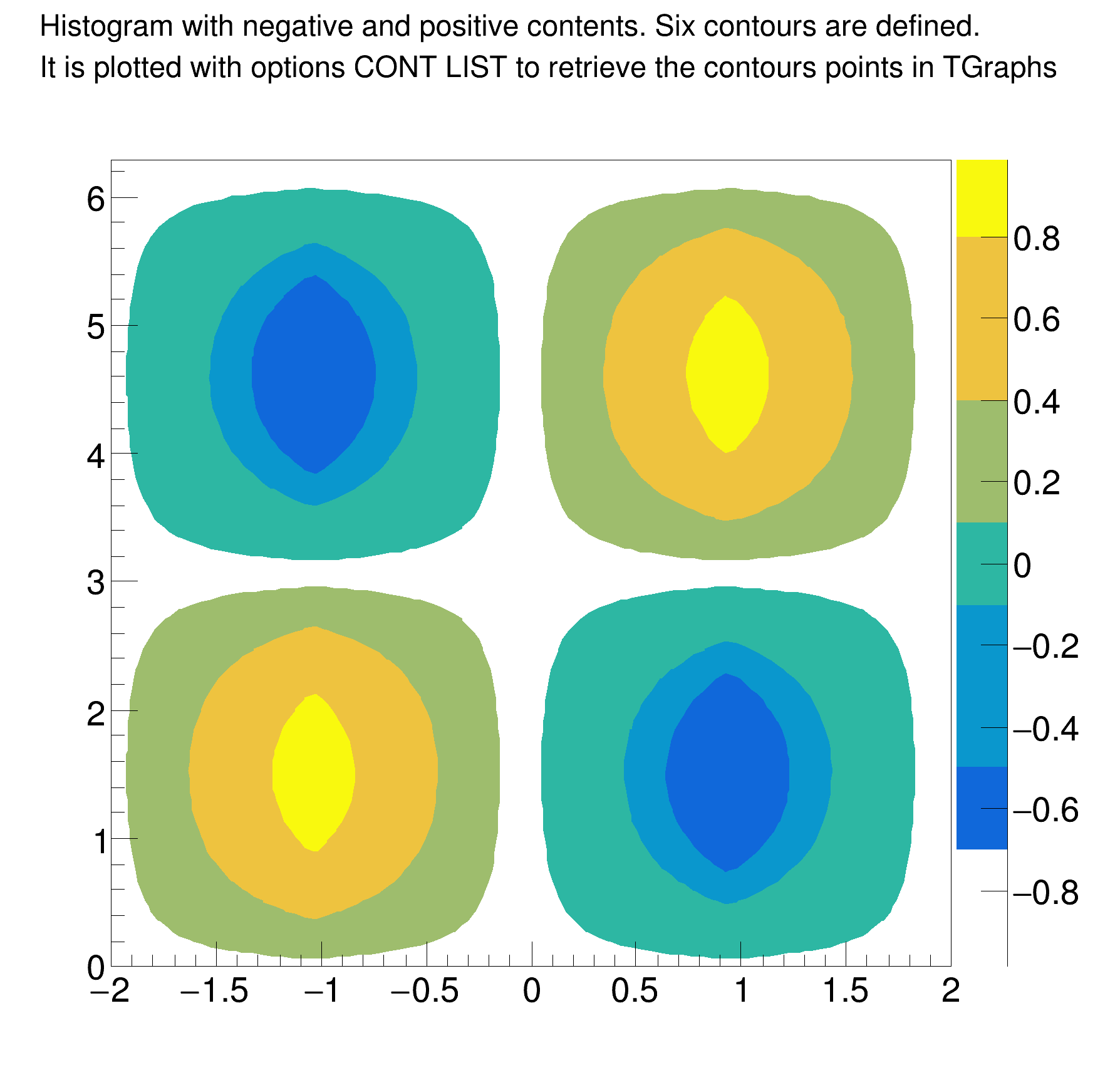
When option LIST is specified together with option CONT, the points used to draw the contours are saved in TGraph objects:
h->Draw("CONT LIST");
gPad->Update();
The contour are saved in TGraph objects once the pad is painted. Therefore to use this functionality in a macro, gPad->Update() should be performed after the histogram drawing. Once the list is built, the contours are accessible in the following way:
TObjArray *contours = gROOT->GetListOfSpecials()->FindObject("contours")
Int_t ncontours     = contours->GetSize();
TList *list         = (TList*)contours->At(i);
Where i is a contour number, and list contains a list of TGraph objects. For one given contour, more than one disjoint polyline may be generated. The number of TGraphs per contour is given by:
list->GetSize();
To access the first graph in the list one should do:
TGraph *gr1 = (TGraph*)list->First();
The following example (ContourList.C) shows how to use this functionality.
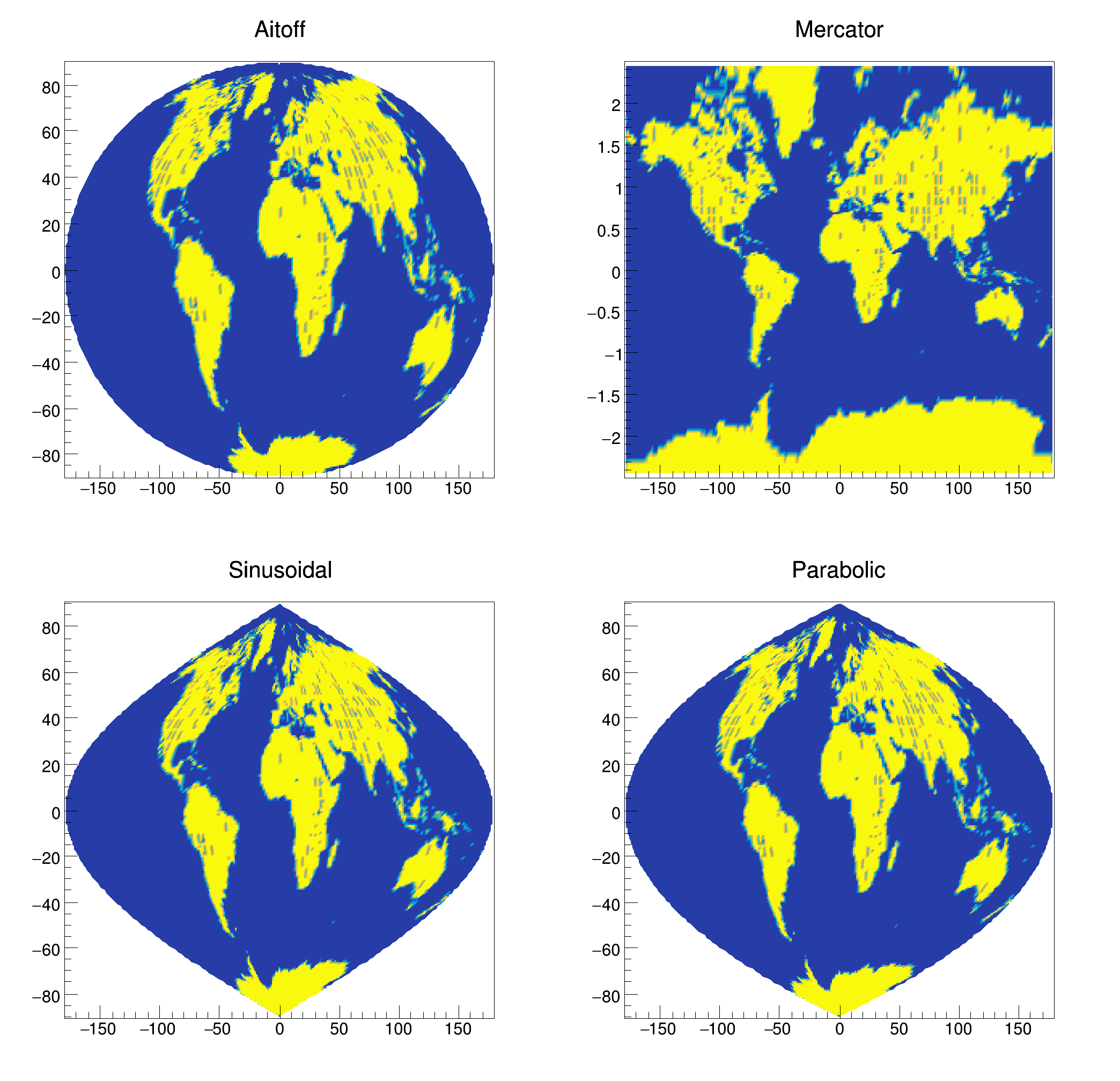
The following options select the CONT4 option and are useful for sky maps or exposure maps (earth.C).
| Option | Description |
|---|---|
| "AITOFF" | Draw a contour via an AITOFF projection. |
| "MERCATOR" | Draw a contour via an Mercator projection. |
| "SINUSOIDAL" | Draw a contour via an Sinusoidal projection. |
| "PARABOLIC" | Draw a contour via an Parabolic projection. |
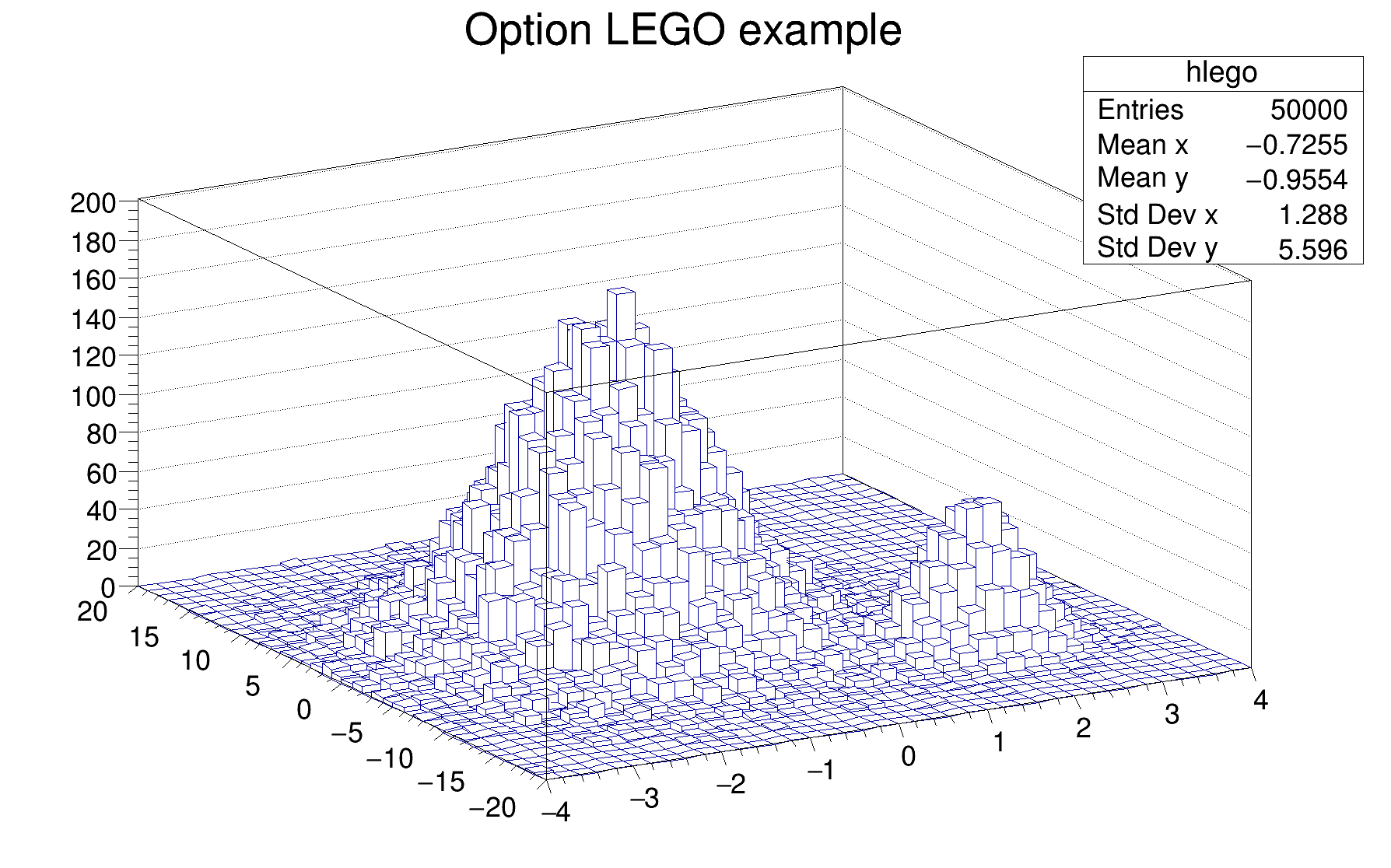
In a lego plot the cell contents are drawn as 3-d boxes. The height of each box is proportional to the cell content. The lego aspect is control with the following options:
| Option | Description |
|---|---|
| "LEGO" | Draw a lego plot using the hidden lines removal technique. |
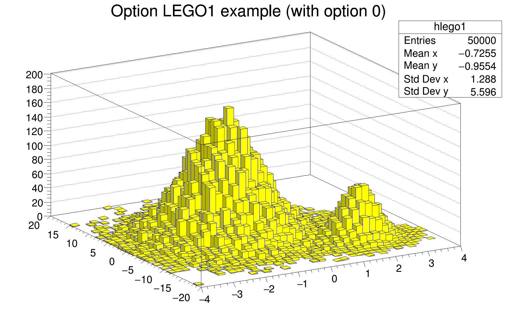
| "LEGO1" | Draw a lego plot using the hidden surface removal technique. |
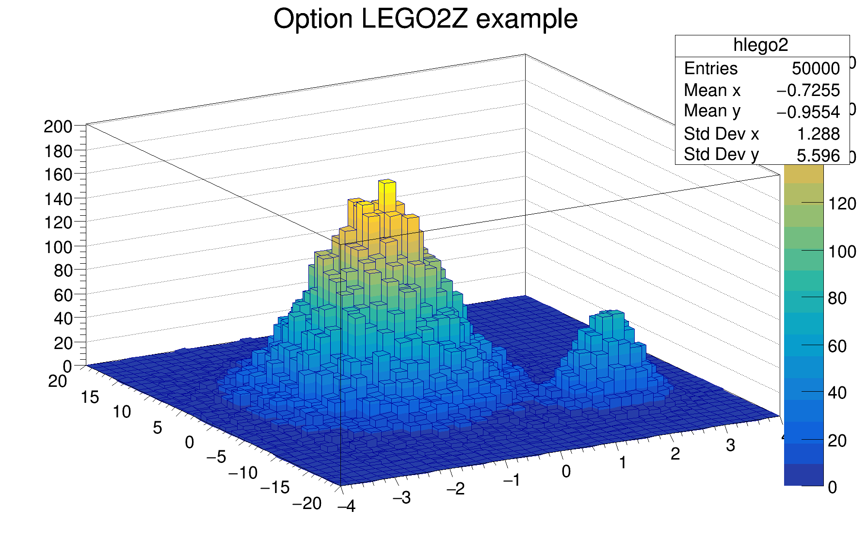
| "LEGO2" | Draw a lego plot using colors to show the cell contents. |
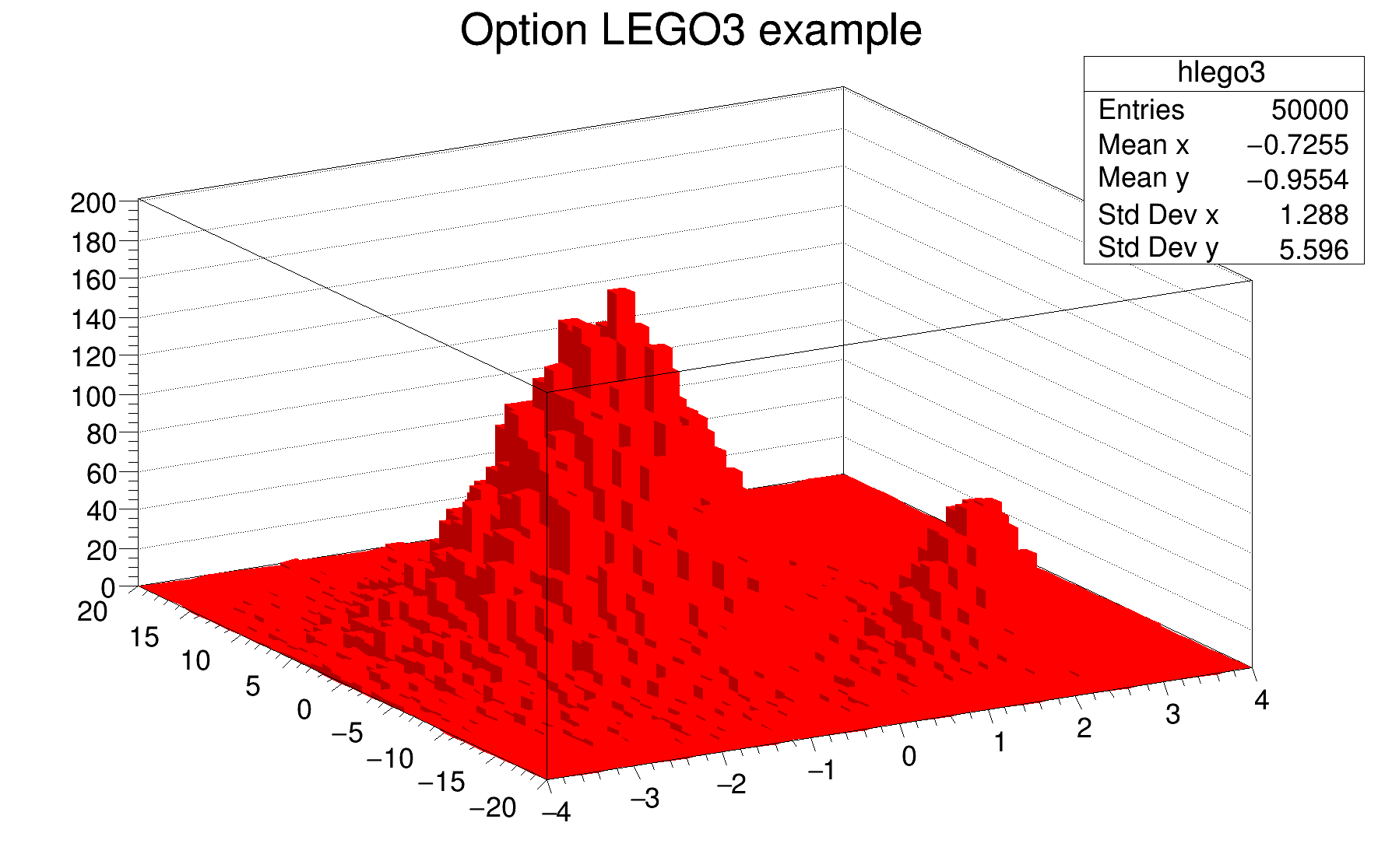
| "LEGO3" | Draw a lego plot with hidden surface removal, like LEGO1 but the border lines of each lego-bar are not drawn. |
| "LEGO4" | Draw a lego plot with hidden surface removal, like LEGO1 but without the shadow effect on each lego-bar. |
| "0" | When used with any LEGO option, the empty bins are not drawn. |
See the limitations with the option "SAME".
Line attributes can be used in lego plots to change the edges' style.
The following example shows a 2D histogram plotted with the option LEGO. The option LEGO draws a lego plot using the hidden lines removal technique.
The following example shows a 2D histogram plotted with the option LEGO1. The option LEGO1 draws a lego plot using the hidden surface removal technique. Combined with any LEGOn option, the option 0 allows to not drawn the empty bins.
The following example shows a 2D histogram plotted with the option LEGO3. Like the option LEGO1, the option LEGO3 draws a lego plot using the hidden surface removal technique but doesn't draw the border lines of each individual lego-bar. This is very useful for histograms having many bins. With such histograms the option LEGO1 gives a black image because of the border lines. This option also works with stacked legos.
The following example shows a 2D histogram plotted with the option LEGO2. The option LEGO2 draws a lego plot using colors to show the cell contents. Combined with the option LEGO2, the option Z allows to display the color palette defined by gStyle->SetPalette().
In a surface plot, cell contents are represented as a mesh. The height of the mesh is proportional to the cell content.
| Option | Description |
|---|---|
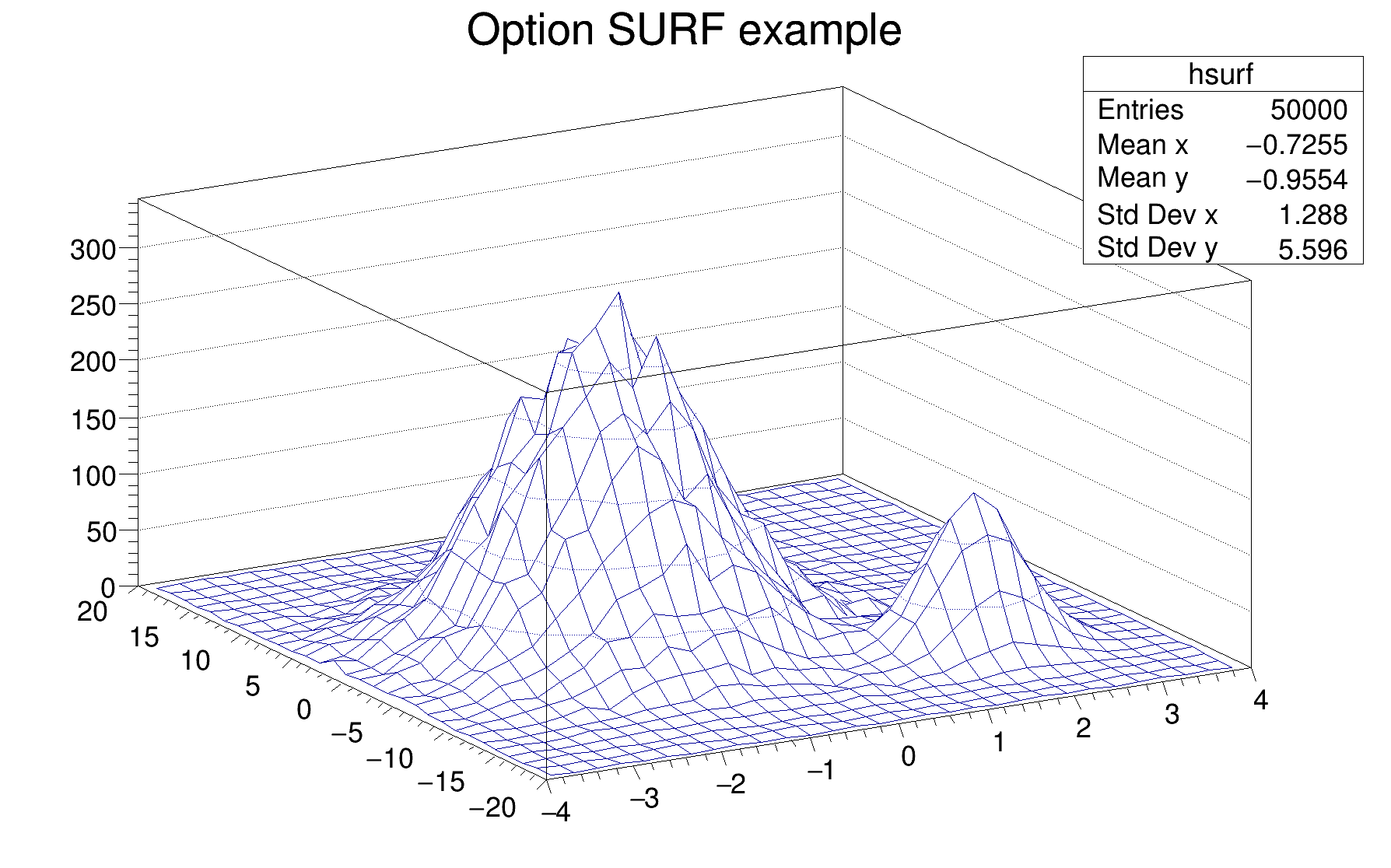
| "SURF" | Draw a surface plot using the hidden line removal technique. |
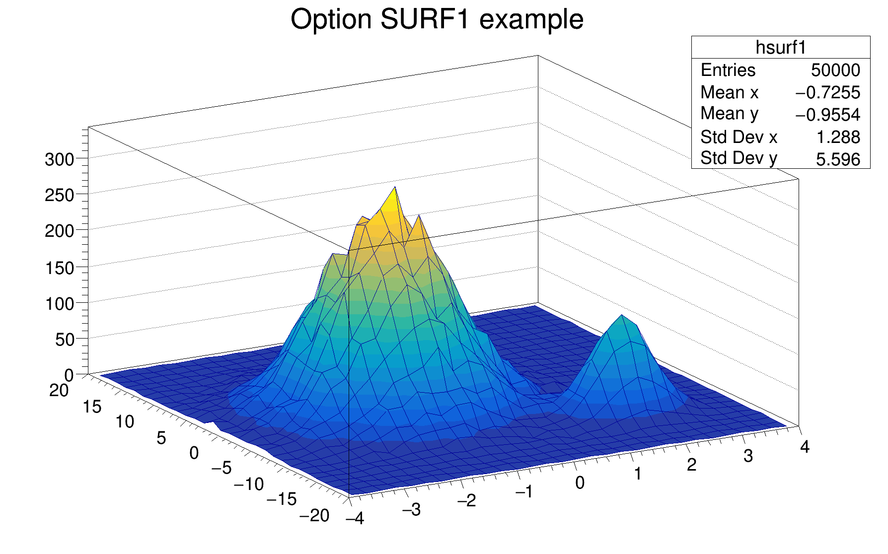
| "SURF1" | Draw a surface plot using the hidden surface removal technique. |
| "SURF2" | Draw a surface plot using colors to show the cell contents. |
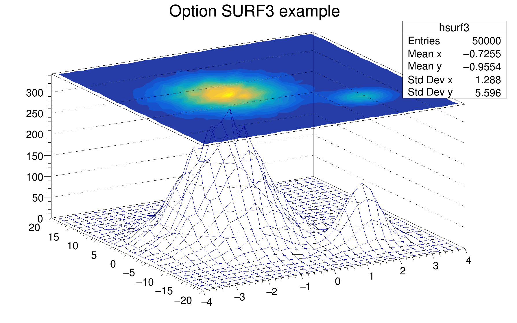
| "SURF3" | Same as SURF with an additional filled contour plot on top. |
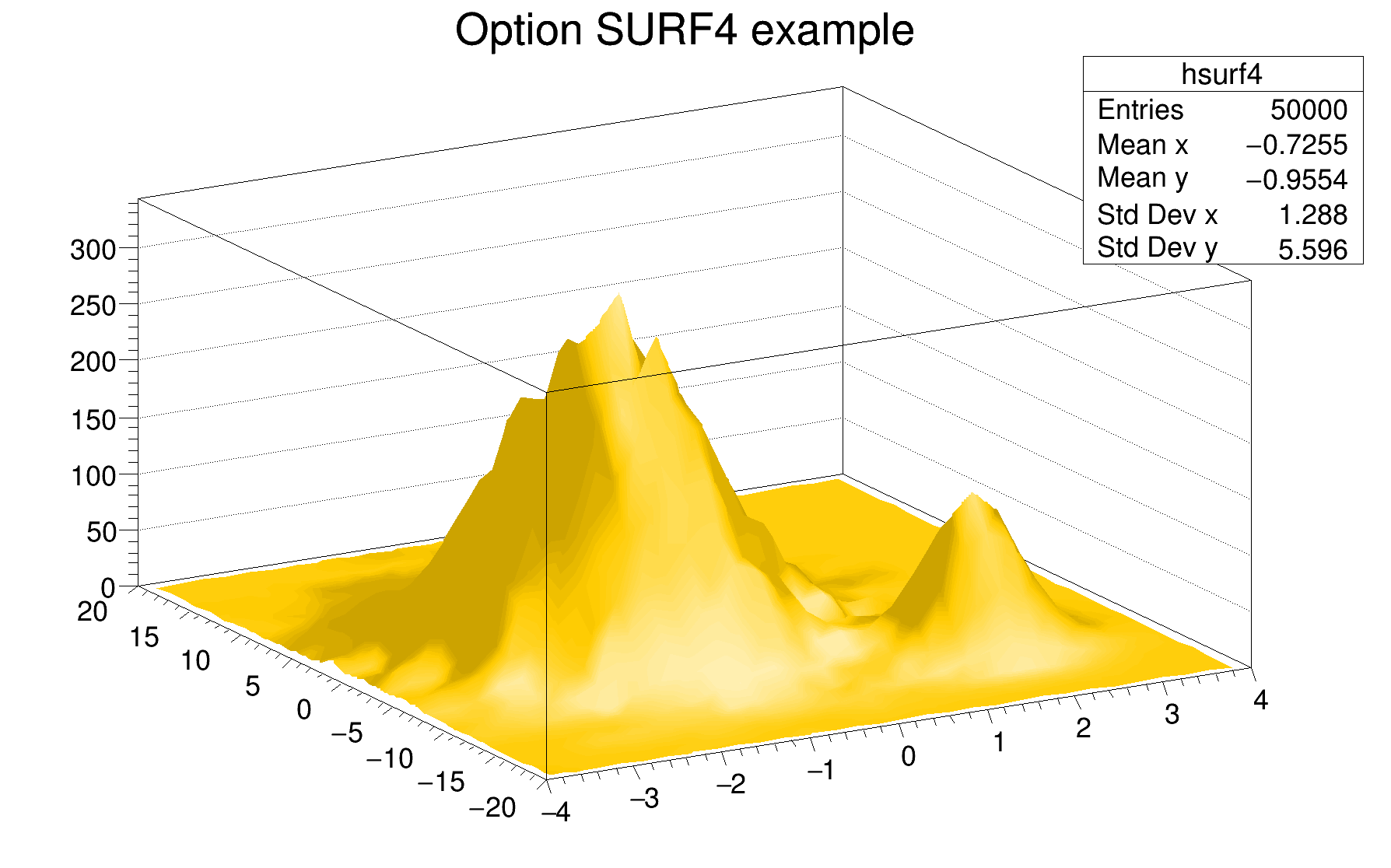
| "SURF4" | Draw a surface using the Gouraud shading technique. |
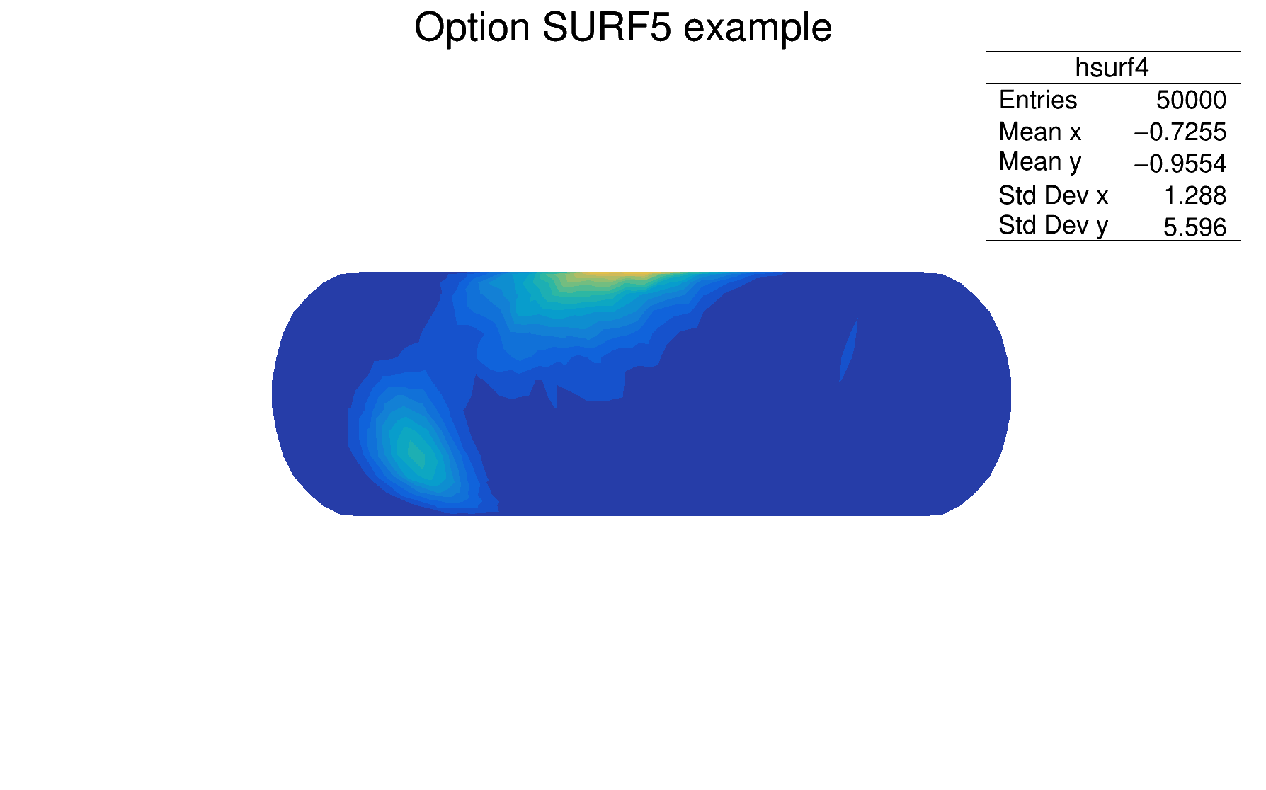
| "SURF5" | Used with one of the options CYL, PSR and CYL this option allows to draw a a filled contour plot. |
| "SURF6" | This option should not be used directly. It is used internally when the CONT is used with option the option SAME on a 3D plot. |
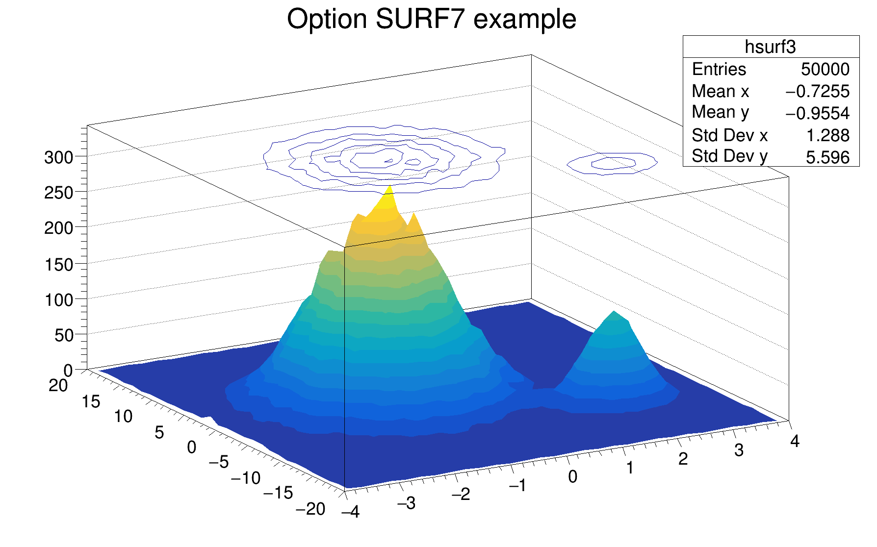
| "SURF7" | Same as SURF2 with an additional line contour plot on top. |
See the limitations with the option "SAME".
The following example shows a 2D histogram plotted with the option SURF. The option SURF draws a lego plot using the hidden lines removal technique.
The following example shows a 2D histogram plotted with the option SURF1. The option SURF1 draws a surface plot using the hidden surface removal technique. Combined with the option SURF1, the option Z allows to display the color palette defined by gStyle->SetPalette().
The following example shows a 2D histogram plotted with the option SURF2. The option SURF2 draws a surface plot using colors to show the cell contents. Combined with the option SURF2, the option Z allows to display the color palette defined by gStyle->SetPalette().

The following example shows a 2D histogram plotted with the option SURF3. The option SURF3 draws a surface plot using the hidden line removal technique with, in addition, a filled contour view drawn on the top. Combined with the option SURF3, the option Z allows to display the color palette defined by gStyle->SetPalette().
The following example shows a 2D histogram plotted with the option SURF4. The option SURF4 draws a surface using the Gouraud shading technique.
The following example shows a 2D histogram plotted with the option SURF5 CYL. Combined with the option SURF5, the option Z allows to display the color palette defined by gStyle->SetPalette().
The following example shows a 2D histogram plotted with the option SURF7. The option SURF7 draws a surface plot using the hidden surfaces removal technique with, in addition, a line contour view drawn on the top. Combined with the option SURF7, the option Z allows to display the color palette defined by gStyle->SetPalette().
As shown in the following example, when a contour plot is painted on top of a surface plot using the option SAME, the contours appear in 3D on the surface.
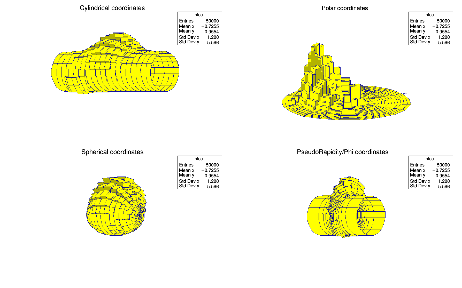
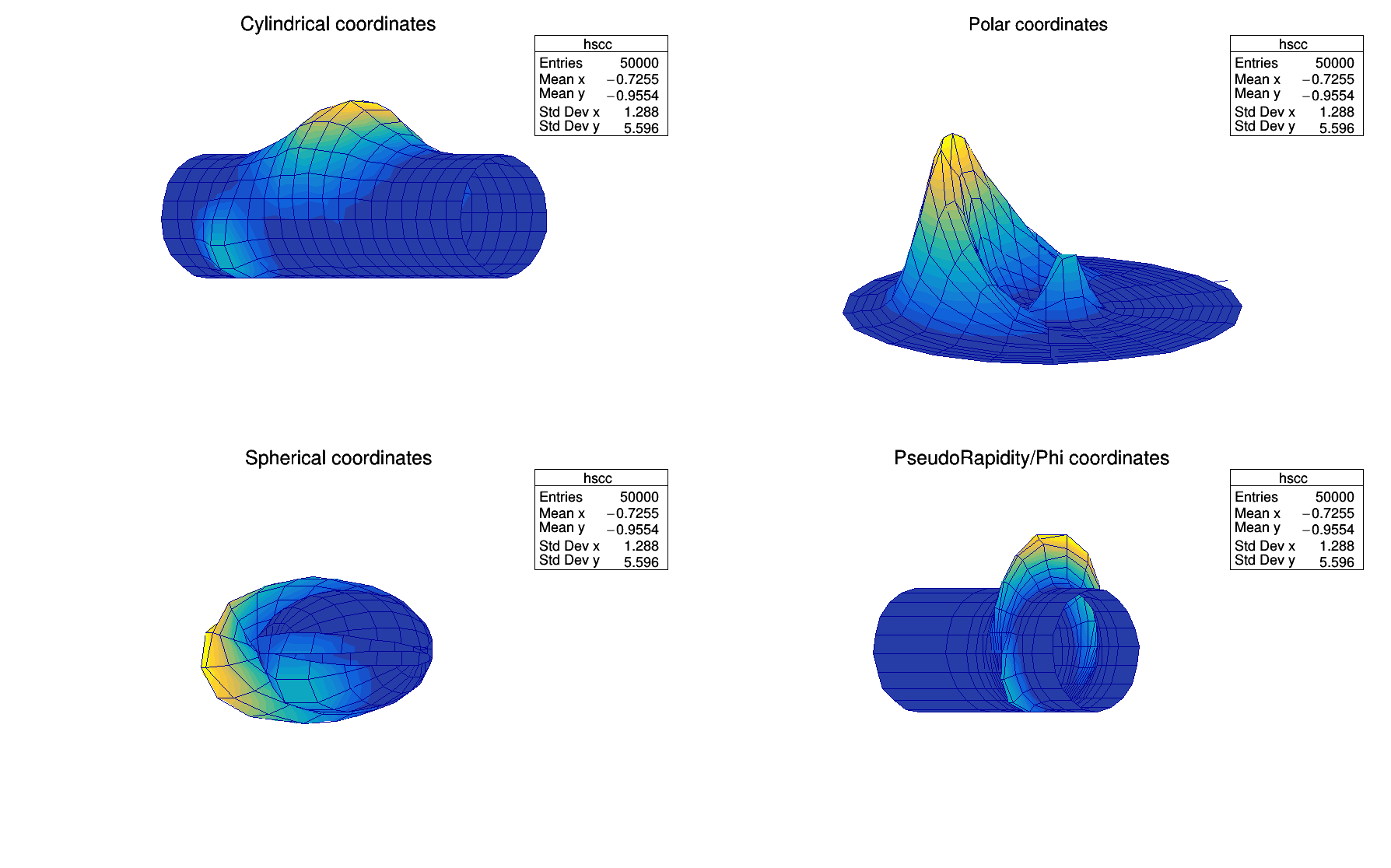
Legos and surfaces plots are represented by default in Cartesian coordinates. Combined with any LEGOn or SURFn options the following options allow to draw a lego or a surface in other coordinates systems.
| Option | Description |
|---|---|
| "CYL" | Use Cylindrical coordinates. The X coordinate is mapped on the angle and the Y coordinate on the cylinder length. |
| "POL" | Use Polar coordinates. The X coordinate is mapped on the angle and the Y coordinate on the radius. |
| "SPH" | Use Spherical coordinates. The X coordinate is mapped on the latitude and the Y coordinate on the longitude. |
| "PSR" | Use PseudoRapidity/Phi coordinates. The X coordinate is mapped on Phi. |
WARNING: Axis are not drawn with these options.
The following example shows the same histogram as a lego plot is the four different coordinates systems.
The following example shows the same histogram as a surface plot is the four different coordinates systems.
By default the base line used to draw the boxes for bar-charts and lego plots is the histogram minimum. It is possible to force this base line to be 0 with the command:
gStyle->SetHistMinimumZero();
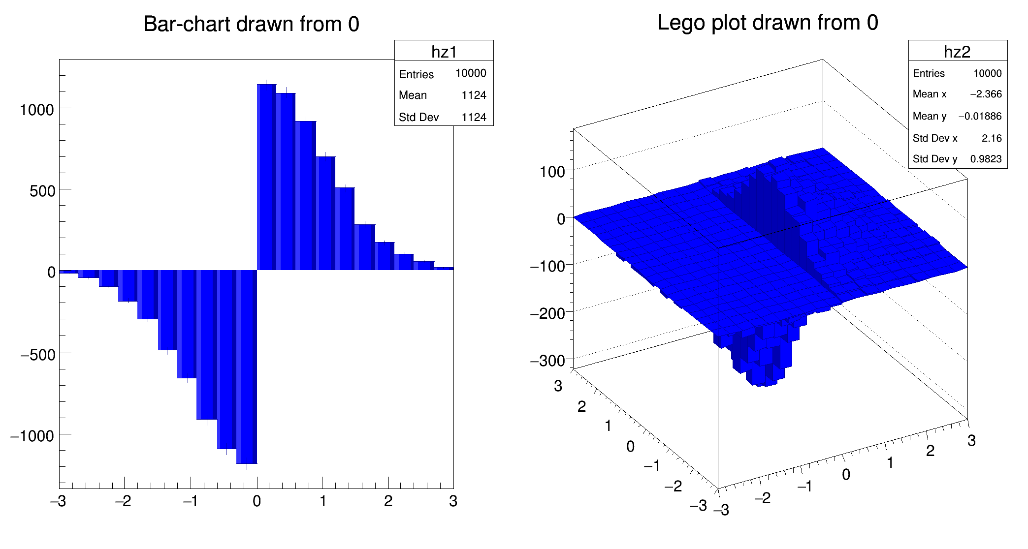
This option also works for horizontal plots. The example given in the section "The bar chart option" appears as follow:
The following options are supported:
| Option | Description |
|---|---|
| "SCAT" | Draw a scatter plot (default). |
| "COL" | Draw a color plot. All the bins are painted even the empty bins. |
| "COLZ" | Same as "COL". In addition the color palette is also drawn. |
| "0" | When used with any COL options, the empty bins are not drawn. |
| "TEXT" | Draw bin contents as text (format set via gStyle->SetPaintTextFormat). |
| "TEXTN" | Draw bin names as text. |
| "TEXTnn" | Draw bin contents as text at angle nn (0 < nn < 90). |
| "L" | Draw the bins boundaries as lines. The lines attributes are the TGraphs ones. |
| "P" | Draw the bins boundaries as markers. The markers attributes are the TGraphs ones. |
| "F" | Draw the bins boundaries as filled polygons. The filled polygons attributes are the TGraphs ones. |
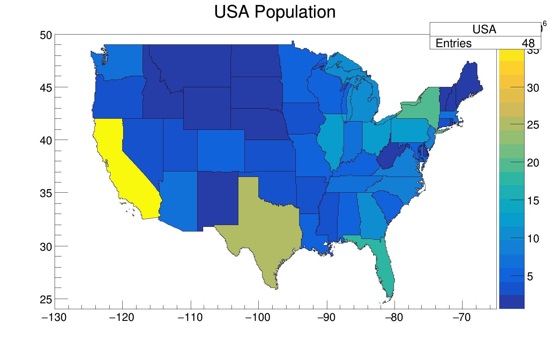
TH2Poly can be drawn as a color plot (option COL). TH2Poly bins can have any shapes. The bins are defined as graphs. The following macro is a very simple example showing how to book a TH2Poly and draw it.
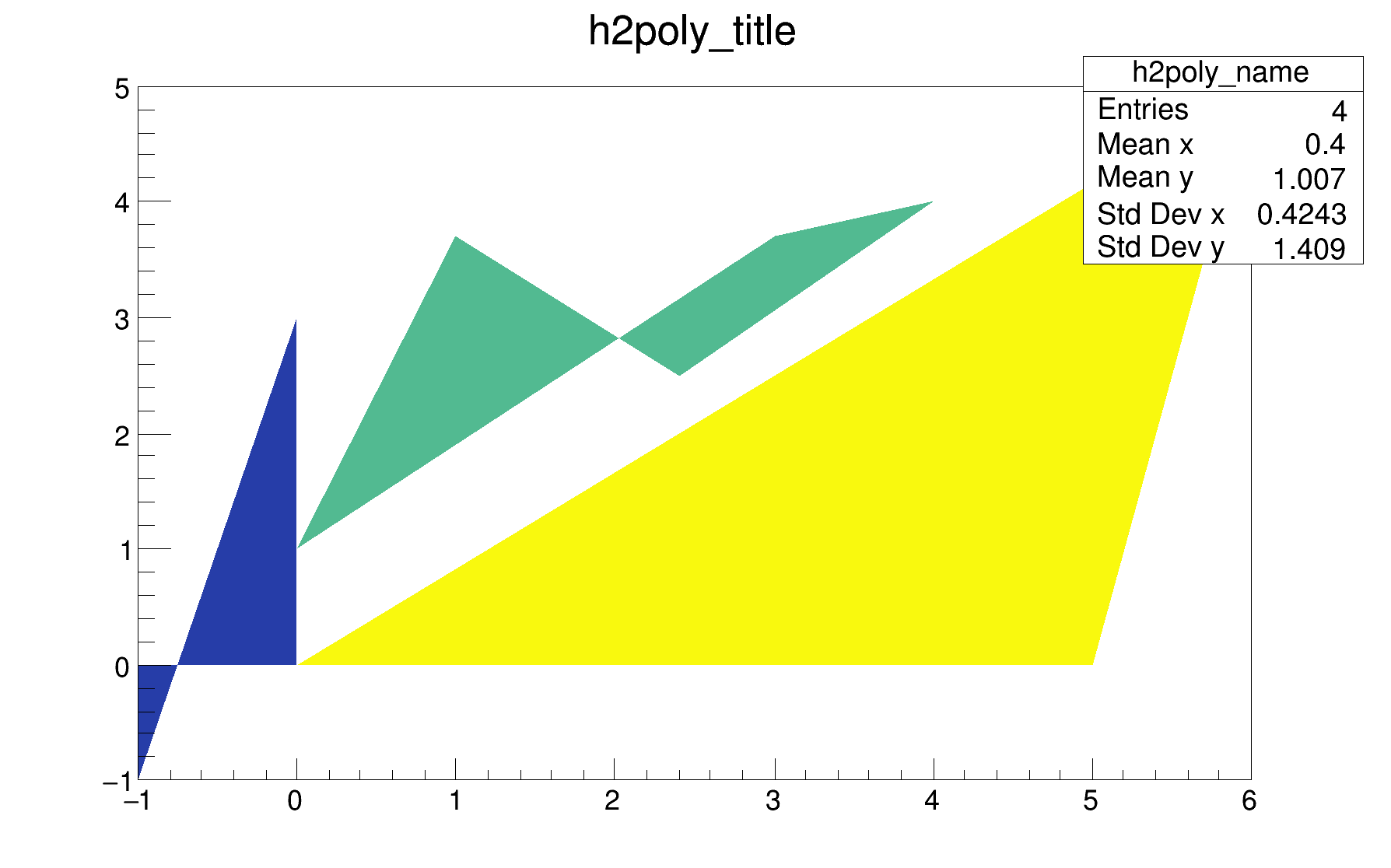
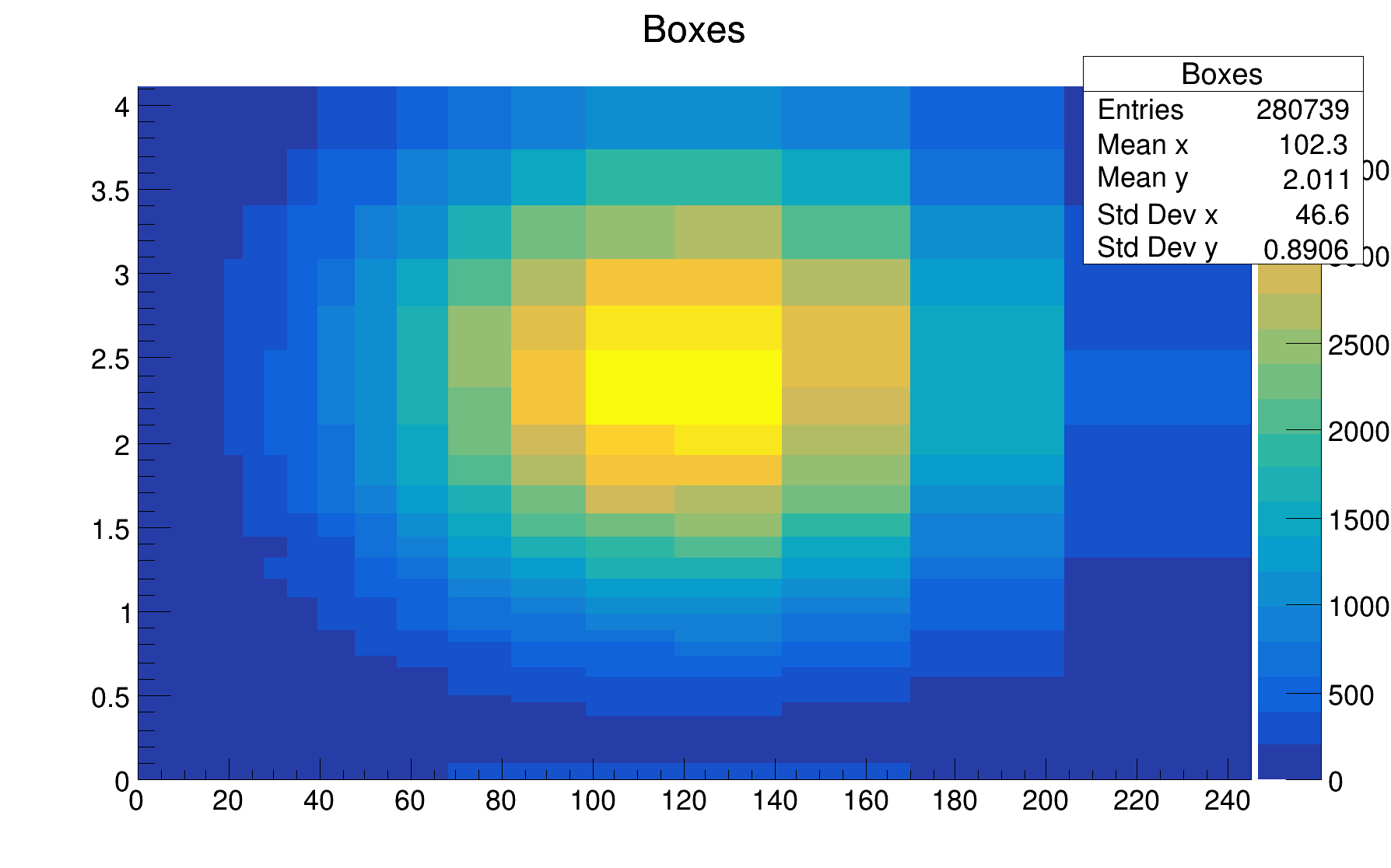
Rectangular bins are a frequent case. The special version of the AddBin method allows to define them more easily like shown in the following example (th2polyBoxes.C).
One TH2Poly bin can be a list of polygons. Such bins are defined by calling AddBin with a TMultiGraph. The following example shows a such case:
TH2Poly histograms can also be plotted using the GL interface using the option "GLLEGO".
In some cases it can be useful to not draw the empty bins. the option "0" combined with the option "COL" et COLZ allows to do that.
This option allows to use the TSpectrum2Painter tools. See the full documentation in TSpectrum2Painter::PaintSpectrum.
When this option is specified, a color palette with an axis indicating the value of the corresponding color is drawn on the right side of the picture. In case, not enough space is left, one can increase the size of the right margin by calling TPad::SetRightMargin(). The attributes used to display the palette axis values are taken from the Z axis of the object. For example, to set the labels size on the palette axis do:
hist->GetZaxis()->SetLabelSize().
WARNING: The palette axis is always drawn vertically.
To change the color palette TStyle::SetPalette should be used, eg:
gStyle->SetPalette(ncolors,colors);
For example the option COL draws a 2D histogram with cells represented by a box filled with a color index which is a function of the cell content. If the cell content is N, the color index used will be the color number in colors[N], etc. If the maximum cell content is greater than ncolors, all cell contents are scaled to ncolors.
If ncolors <= 0, a default palette (see below) of 50 colors is defined. This palette is recommended for pads, labels ...
if ncolors == 1 && colors == 0, then a Pretty Palette with a Spectrum Violet->Red is created with 50 colors. That's the default rain bow palette.
Other pre-defined palettes with 255 colors are available when colors == 0. The following value of ncolors give access to:
if ncolors = 51 and colors=0, a Deep Sea palette is used.
if ncolors = 52 and colors=0, a Grey Scale palette is used.
if ncolors = 53 and colors=0, a Dark Body Radiator palette is used.
if ncolors = 54 and colors=0, a two-color hue palette palette is used.(dark blue through neutral gray to bright yellow)
if ncolors = 55 and colors=0, a Rain Bow palette is used.
if ncolors = 56 and colors=0, an inverted Dark Body Radiator palette is used.
If ncolors > 0 && colors == 0, the default palette is used with a maximum of ncolors.
The default palette defines:
The color numbers specified in the palette can be viewed by selecting the item colors in the VIEW menu of the canvas tool bar. The red, green, and blue components of a color can be changed thanks to TColor::SetRGB().
Using a TCutG object, it is possible to draw a sub-range of a 2D histogram. One must create a graphical cut (mouse or C++) and specify the name of the cut between [] in the Draw() option. For example (fit2a.C), with a TCutG named cutg, one can call:
myhist->Draw("surf1 [cutg]");
To invert the cut, it is enough to put a - in front of its name:
myhist->Draw("surf1 [-cutg]");
It is possible to apply several cuts (, means logical AND):
myhist->Draw("surf1 [cutg1,cutg2]");
| Option | Description |
|---|---|
| "ISO" | Draw a Gouraud shaded 3d iso surface through a 3d histogram. It paints one surface at the value computed as follow: SumOfWeights/(NbinsX*NbinsY*NbinsZ) |
| "BOX" | Draw a for each cell with volume proportional to the content's absolute value. An hidden line removal algorithm is used |
| "BOX1" | Same as BOX but an hidden surface removal algorithm is used |
| "BOX2" | The boxes' colors are picked in the current palette according to the bins' contents |
| "BOX2Z" | Same as "BOX2". In addition the color palette is also drawn. |
| "BOX3" | Same as BOX1, but the border lines of each lego-bar are not drawn. |
Note that instead of BOX one can also use LEGO.
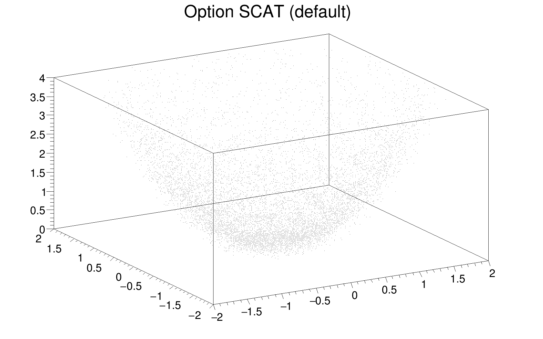
By default, like 2D histograms, 3D histograms are drawn as scatter plots.
The following example shows a 3D histogram plotted as a scatter plot.
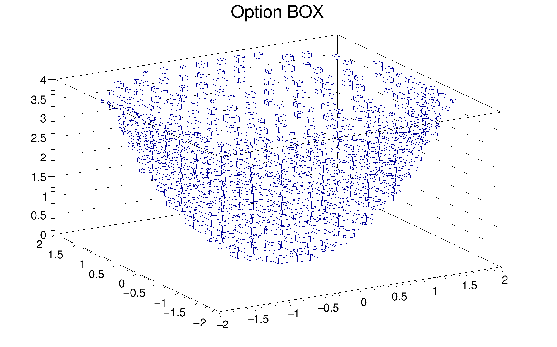
The following example shows a 3D histogram plotted with the option BOX.
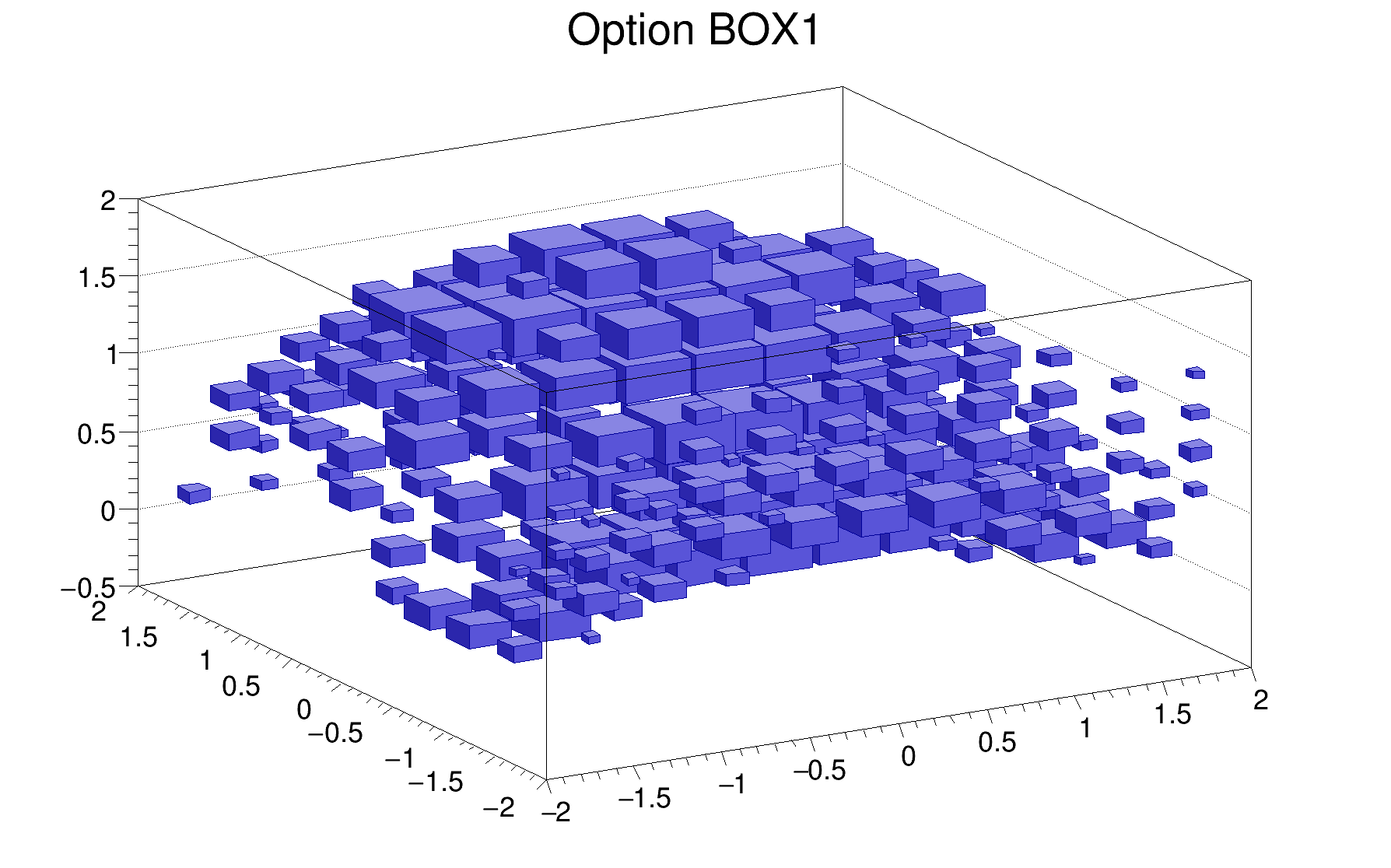
The following example shows a 3D histogram plotted with the option BOX1.
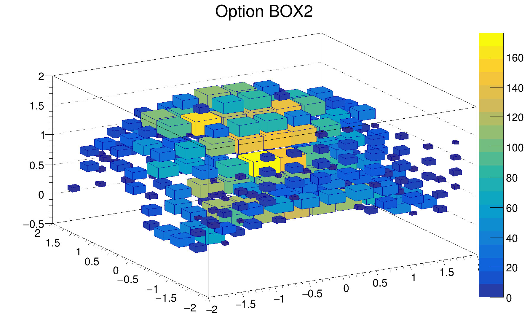
The following example shows a 3D histogram plotted with the option BOX2.
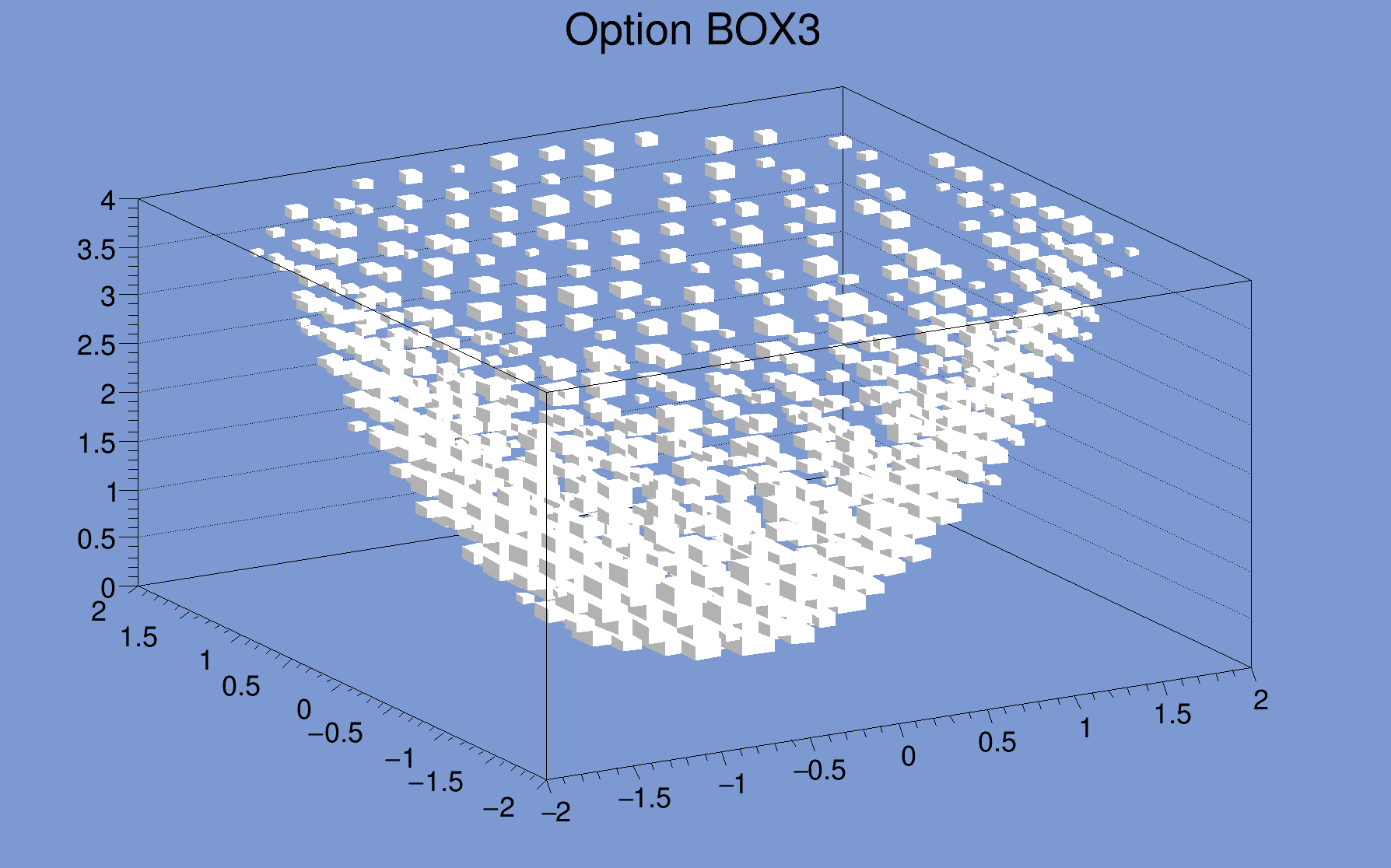
The following example shows a 3D histogram plotted with the option BOX3.
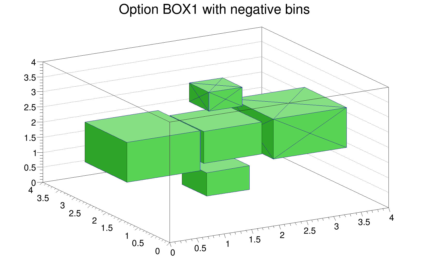
For all the BOX options each bin is drawn as a 3D box with a volume proportional to the absolute value of the bin content. The bins with a negative content are drawn with a X on each face of the box as shown in the following example:
The following example shows a 3D histogram plotted with the option ISO.
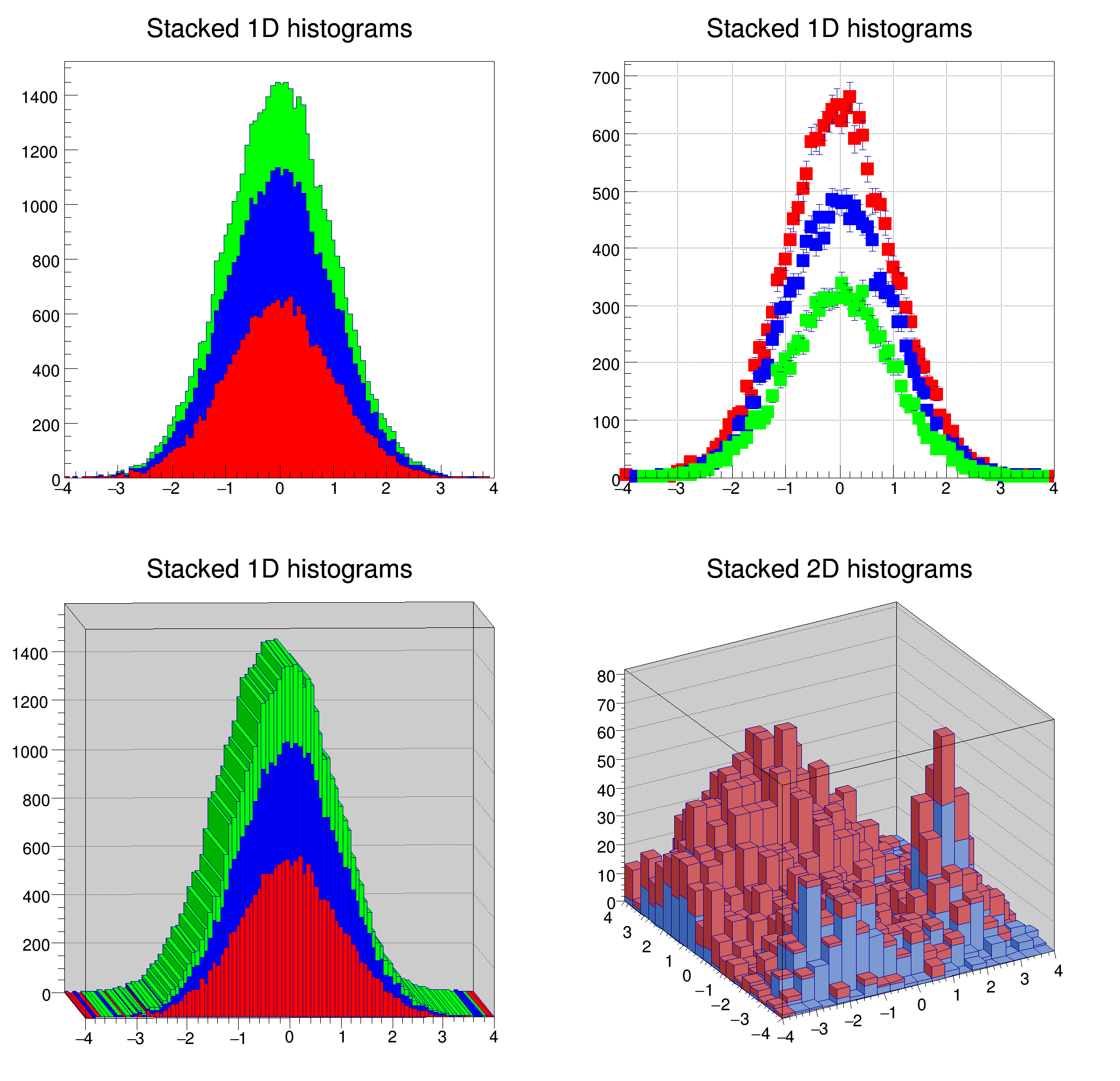
Stacks of histograms are managed with the THStack. A THStack is a collection of TH1 (or derived) objects. For painting only the THStack containing TH1 only or THStack containing TH2 only will be considered.
By default, histograms are shown stacked:
If the option NOSTACK is specified, the histograms are all paint in the same pad as if the option SAME had been specified. This allows to compute X and Y scales common to all the histograms, like TMultiGraph does for graphs.
If the option PADS is specified, the current pad/canvas is subdivided into a number of pads equal to the number of histograms and each histogram is paint into a separate pad.
The following example shows various types of stacks (hstack.C).
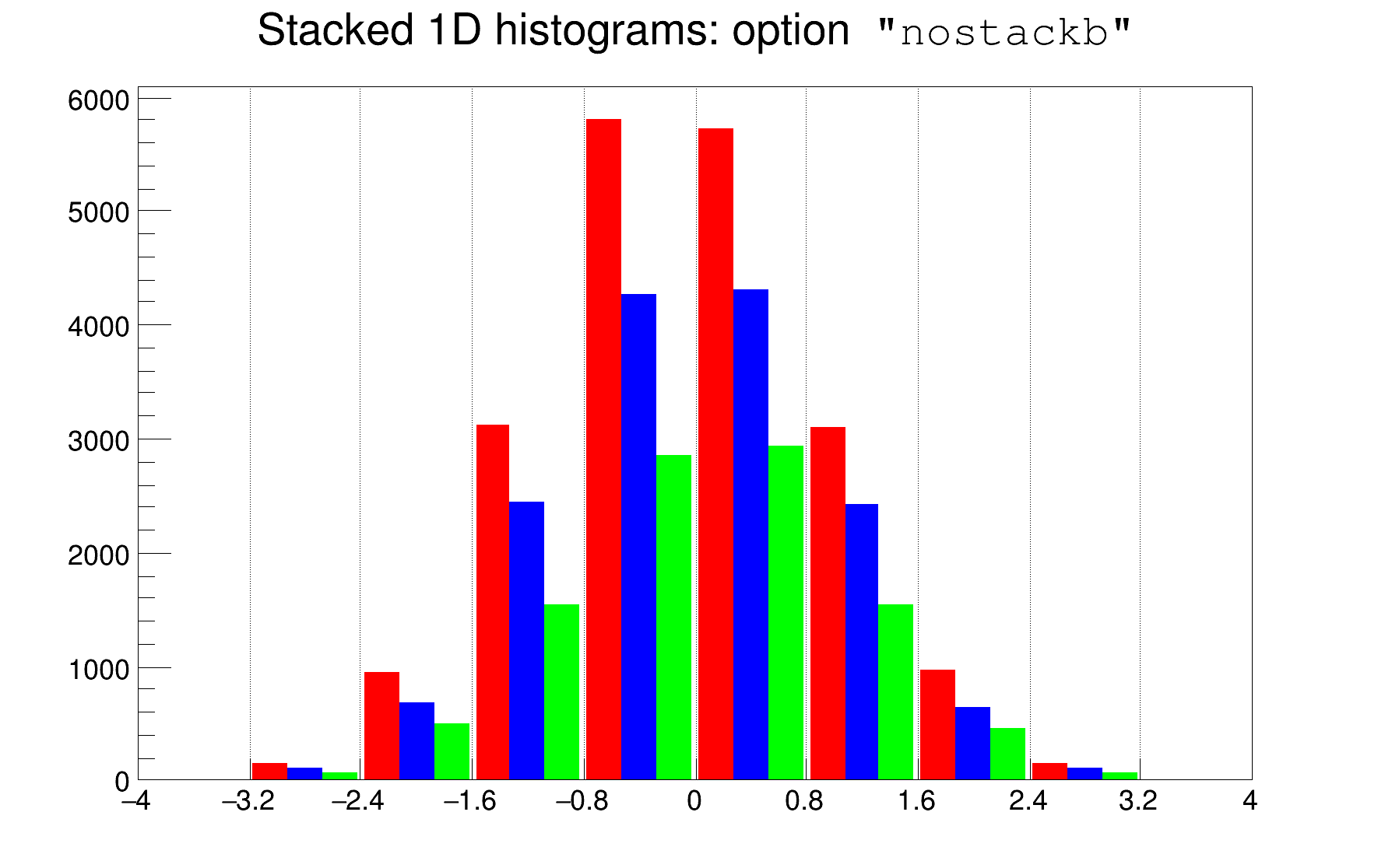
The option nostackb allows to draw the histograms next to each other as bar charts:
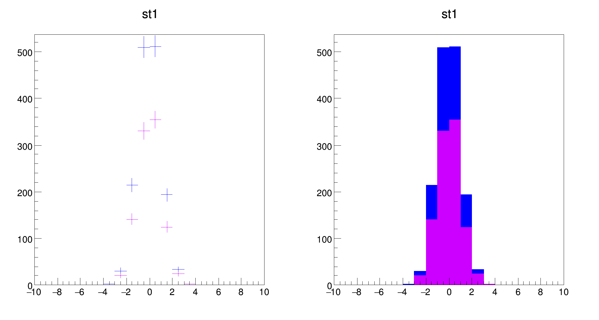
If at least one of the histograms in the stack has errors, the whole stack is visualized by default with error bars. To visualize it without errors the option HIST should be used.
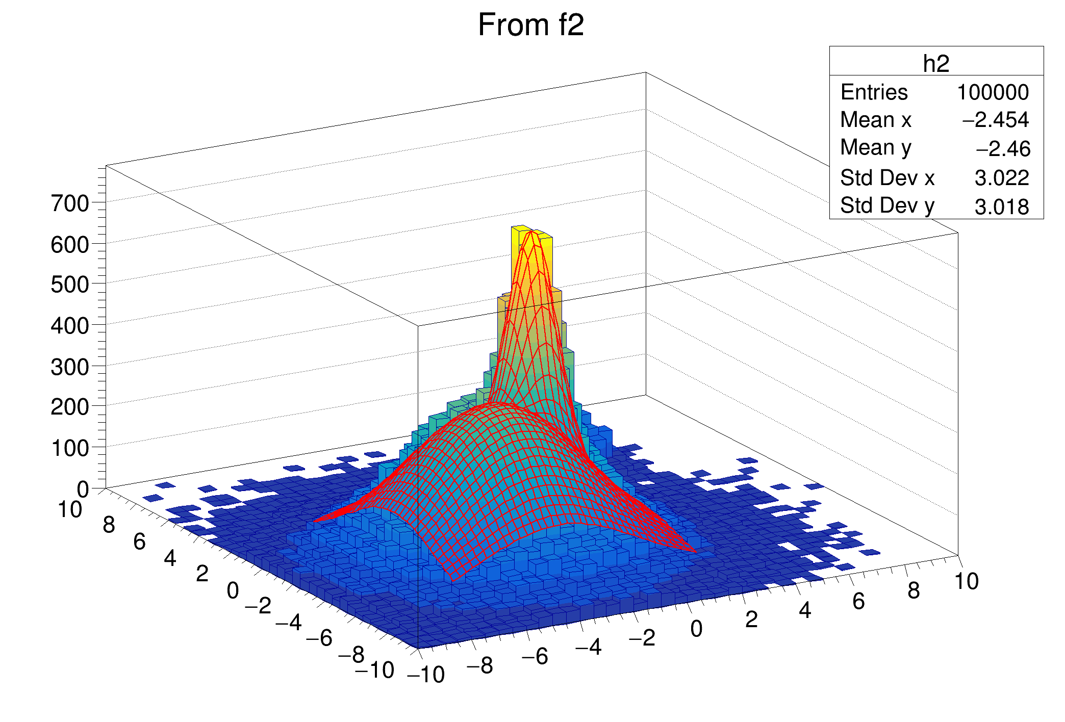
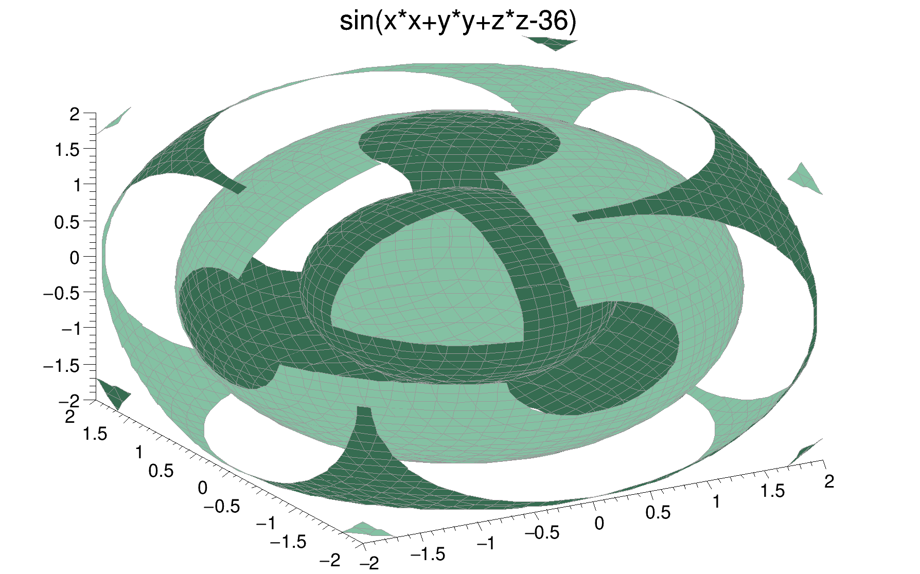
3D implicit functions (TF3) can be drawn as iso-surfaces. The implicit function f(x,y,z) = 0 is drawn in cartesian coordinates. In the following example the options "FB" and "BB" suppress the "Front Box" and "Back Box" around the plot.
An associated function is created by TH1::Fit. More than on fitted function can be associated with one histogram (see TH1::Fit).
A TF1 object f1 can be added to the list of associated functions of an histogram h without calling TH1::Fit simply doing:
h->GetListOfFunctions()->Add(f1);
or
h->GetListOfFunctions()->Add(f1,someoption);
To retrieve a function by name from this list, do:
TF1 *f1 = (TF1*)h->GetListOfFunctions()->FindObject(name);
or
TF1 *f1 = h->GetFunction(name);
Associated functions are automatically painted when an histogram is drawn. To avoid the painting of the associated functions the option HIST should be added to the list of the options used to paint the histogram.
The class TGLHistPainter allows to paint data set using the OpenGL 3D graphics library. The plotting options start with GL keyword. In addition, in order to inform canvases that OpenGL should be used to render 3D representations, the following option should be set:
gStyle->SetCanvasPreferGL(true);
The following types of plots are provided:
For lego plots the supported options are:
| Option | Description |
|---|---|
| "GLLEGO" | Draw a lego plot. It works also for TH2Poly. |
| "GLLEGO2" | Bins with color levels. |
| "GLLEGO3" | Cylindrical bars. |
Lego painter in cartesian supports logarithmic scales for X, Y, Z. In polar only Z axis can be logarithmic, in cylindrical only Y.
For surface plots (TF2 and TH2) the supported options are:
| Option | Description |
|---|---|
| "GLSURF" | Draw a surface. |
| "GLSURF1" | Surface with color levels |
| "GLSURF2" | The same as "GLSURF1" but without polygon outlines. |
| "GLSURF3" | Color level projection on top of plot (works only in cartesian coordinate system). |
| "GLSURF4" | Same as "GLSURF" but without polygon outlines. |
The surface painting in cartesian coordinates supports logarithmic scales along X, Y, Z axis. In polar coordinates only the Z axis can be logarithmic, in cylindrical coordinates only the Y axis.
Additional options to SURF and LEGO - Coordinate systems:
| Option | Description |
|---|---|
| " " | Default, cartesian coordinates system. |
| "POL" | Polar coordinates system. |
| "CYL" | Cylindrical coordinates system. |
| "SPH" | Spherical coordinates system. |
The supported option is:
| Option | Description |
|---|---|
| "GLCOL" | H3 is drawn using semi-transparent colored boxes. See $ROOTSYS/tutorials/gl/glvox1.C. |
The supported options are:
| Option | Description |
|---|---|
| "GLBOX" | TH3 as a set of boxes, size of box is proportional to bin content. |
| "GLBOX1" | The same as "glbox", but spheres are drawn instead of boxes. |
The supported option is:
| Option | Description |
|---|---|
| "GLISO" | TH3 is drawn using iso-surfaces. |
The supported option is:
| Option | Description |
|---|---|
| "GLTF3" | Draw a TF3. |
$ROOTSYS/tutorials/gl/glparametric.C shows how to create parametric equations and visualize the surface.
All the interactions are implemented via standard methods DistancetoPrimitive() and ExecuteEvent(). That's why all the interactions with the OpenGL plots are possible only when the mouse cursor is in the plot's area (the plot's area is the part of a the pad occupied by gl-produced picture). If the mouse cursor is not above gl-picture, the standard pad interaction is performed.
Different parts of the plot can be selected:
The selected plot can be moved in a pad's area by pressing and holding the left mouse button and the shift key.
Surface, iso, box, TF3 and parametric painters support box cut by pressing the 'c' or 'C' key when the mouse cursor is in a plot's area. That will display a transparent box, cutting away part of the surface (or boxes) in order to show internal part of plot. This box can be moved inside the plot's area (the full size of the box is equal to the plot's surrounding box) by selecting one of the box cut axes and pressing the left mouse button to move it.
Currently, all gl-plots support some form of slicing. When back plane is selected (and if it's highlighted in green) you can press and hold left mouse button and shift key and move this back plane inside plot's area, creating the slice. During this "slicing" plot becomes semi-transparent. To remove all slices (and projected curves for surfaces) double click with left mouse button in a plot's area.
The surface profile is displayed on the slicing plane. The profile projection is drawn on the back plane by pressing 'p' or 'P' key.
The contour plot is drawn on the slicing plane. For TF3 the color scheme can be changed by pressing 's' or 'S'.
The contour plot corresponding to slice plane position is drawn in real time.
Slicing is similar to "GLBOX" option.
No slicing. Additional keys: 's' or 'S' to change color scheme - about 20 color schemes supported ('s' for "scheme"); 'l' or 'L' to increase number of polygons ('l' for "level" of details), 'w' or 'W' to show outlines ('w' for "wireframe").
Definition at line 47 of file THistPainter.h.
Public Member Functions | |
| THistPainter () | |
| Default constructor. More... | |
| virtual | ~THistPainter () |
| Default destructor. More... | |
| virtual std::vector< THistRenderingRegion > | ComputeRenderingRegions (TAxis *pAxis, Int_t nPixels, bool isLog) |
| Returns the rendering regions for an axis to use in the COL2 option. More... | |
| virtual void | DefineColorLevels (Int_t ndivz) |
| Define the color levels used to paint legos, surfaces etc.. More... | |
| virtual Int_t | DistancetoPrimitive (Int_t px, Int_t py) |
| Compute the distance from the point px,py to a line. More... | |
| virtual void | DrawPanel () |
| Display a panel with all histogram drawing options. More... | |
| virtual void | ExecuteEvent (Int_t event, Int_t px, Int_t py) |
Execute the actions corresponding to event. More... | |
| virtual TList * | GetContourList (Double_t contour) const |
| Get a contour (as a list of TGraphs) using the Delaunay triangulation. More... | |
| virtual char * | GetObjectInfo (Int_t px, Int_t py) const |
| Display the histogram info (bin number, contents, integral up to bin corresponding to cursor position px,py. More... | |
| virtual TList * | GetStack () const |
| virtual Bool_t | IsInside (Int_t x, Int_t y) |
Return kTRUE if the cell ix, iy is inside one of the graphical cuts. More... | |
| virtual Bool_t | IsInside (Double_t x, Double_t y) |
Return kTRUE if the point x, y is inside one of the graphical cuts. More... | |
| virtual Int_t | MakeChopt (Option_t *option) |
Decode string choptin and fill Hoption structure. More... | |
| virtual Int_t | MakeCuts (char *cutsopt) |
Decode string choptin and fill Graphical cuts structure. More... | |
| virtual void | Paint (Option_t *option="") |
| Control routine to paint any kind of histograms More... | |
| virtual void | Paint2DErrors (Option_t *option) |
| Draw 2D histograms errors. More... | |
| virtual void | PaintArrows (Option_t *option) |
| Control function to draw a table as an arrow plot More... | |
| virtual void | PaintAxis (Bool_t drawGridOnly=kFALSE) |
| Draw axis (2D case) of an histogram. More... | |
| virtual void | PaintBar (Option_t *option) |
| Draw a bar-chart in a normal pad. More... | |
| virtual void | PaintBarH (Option_t *option) |
| Draw a bar char in a rotated pad (X vertical, Y horizontal) More... | |
| virtual void | PaintBoxes (Option_t *option) |
| Control function to draw a 2D histogram as a box plot More... | |
| virtual void | PaintCandlePlot (Option_t *option) |
| Control function to draw a 2D histogram as a candle (box) plot or violin plot More... | |
| virtual void | PaintColorLevels (Option_t *option) |
| Control function to draw a 2D histogram as a color plot. More... | |
| virtual void | PaintColorLevelsFast (Option_t *option) |
| Rendering scheme for the COL2 and COLZ2 options More... | |
| virtual void | PaintContour (Option_t *option) |
| Control function to draw a 2D histogram as a contour plot. More... | |
| virtual Int_t | PaintContourLine (Double_t elev1, Int_t icont1, Double_t x1, Double_t y1, Double_t elev2, Int_t icont2, Double_t x2, Double_t y2, Double_t *xarr, Double_t *yarr, Int_t *itarr, Double_t *levels) |
Fill the matrix xarr and yarr for Contour Plot. More... | |
| virtual void | PaintErrors (Option_t *option) |
| Draw 1D histograms error bars. More... | |
| virtual void | PaintFrame () |
| Calculate range and clear pad (canvas). More... | |
| virtual void | PaintFunction (Option_t *option) |
| Paint functions associated to an histogram. More... | |
| virtual void | PaintH3 (Option_t *option="") |
| Control function to draw a 3D histograms. More... | |
| virtual void | PaintH3Box (Int_t iopt) |
| Control function to draw a 3D histogram with boxes. More... | |
| virtual void | PaintH3BoxRaster () |
| Control function to draw a 3D histogram with boxes. More... | |
| virtual void | PaintH3Iso () |
| Control function to draw a 3D histogram with Iso Surfaces. More... | |
| virtual void | PaintHist (Option_t *option) |
| Control routine to draw 1D histograms More... | |
| virtual Int_t | PaintInit () |
| Compute histogram parameters used by the drawing routines. More... | |
| virtual Int_t | PaintInitH () |
| Compute histogram parameters used by the drawing routines for a rotated pad. More... | |
| virtual void | PaintLego (Option_t *option) |
| Control function to draw a 2D histogram as a lego plot. More... | |
| virtual void | PaintLegoAxis (TGaxis *axis, Double_t ang) |
| Draw the axis for legos and surface plots. More... | |
| virtual void | PaintPalette () |
| Paint the color palette on the right side of the pad. More... | |
| virtual void | PaintScatterPlot (Option_t *option) |
| Control function to draw a 2D histogram as a scatter plot. More... | |
| virtual void | PaintStat (Int_t dostat, TF1 *fit) |
| Draw the statistics box for 1D and profile histograms. More... | |
| virtual void | PaintStat2 (Int_t dostat, TF1 *fit) |
| Draw the statistics box for 2D histograms. More... | |
| virtual void | PaintStat3 (Int_t dostat, TF1 *fit) |
| Draw the statistics box for 3D histograms. More... | |
| virtual void | PaintSurface (Option_t *option) |
| Control function to draw a 2D histogram as a surface plot. More... | |
| virtual void | PaintTable (Option_t *option) |
| Control function to draw 2D/3D histograms (tables). More... | |
| virtual void | PaintText (Option_t *option) |
| Control function to draw a 1D/2D histograms with the bin values. More... | |
| virtual void | PaintTF3 () |
| Control function to draw a 3D implicit functions. More... | |
| virtual void | PaintTH2PolyBins (Option_t *option) |
| Control function to draw a TH2Poly bins' contours. More... | |
| virtual void | PaintTH2PolyColorLevels (Option_t *option) |
| Control function to draw a TH2Poly as a color plot. More... | |
| virtual void | PaintTH2PolyScatterPlot (Option_t *option) |
| Control function to draw a TH2Poly as a scatter plot. More... | |
| virtual void | PaintTH2PolyText (Option_t *option) |
| Control function to draw a TH2Poly as a text plot. More... | |
| virtual void | PaintTitle () |
| Draw the histogram title. More... | |
| virtual void | PaintTriangles (Option_t *option) |
| Control function to draw a table using Delaunay triangles. More... | |
| virtual void | ProcessMessage (const char *mess, const TObject *obj) |
Process message mess. More... | |
| virtual void | RecalculateRange () |
| Recompute the histogram range following graphics operations. More... | |
| virtual void | RecursiveRemove (TObject *) |
| Recursively remove this object from a list. More... | |
| virtual void | SetHistogram (TH1 *h) |
Set current histogram to h More... | |
| virtual void | SetShowProjection (const char *option, Int_t nbins) |
| Set projection. More... | |
| virtual void | SetStack (TList *stack) |
| virtual void | ShowProjection3 (Int_t px, Int_t py) |
Show projection (specified by fShowProjection) of a TH3. More... | |
| virtual void | ShowProjectionX (Int_t px, Int_t py) |
| Show projection onto X. More... | |
| virtual void | ShowProjectionY (Int_t px, Int_t py) |
| Show projection onto Y. More... | |
| virtual Int_t | TableInit () |
| Initialize various options to draw 2D histograms. More... | |
 Public Member Functions inherited from TVirtualHistPainter Public Member Functions inherited from TVirtualHistPainter | |
| TVirtualHistPainter () | |
| virtual | ~TVirtualHistPainter () |
| Public Member Functions inherited from TObject | |
| TObject () | |
| TObject constructor. More... | |
| TObject (const TObject &object) | |
| TObject copy ctor. More... | |
| virtual | ~TObject () |
| TObject destructor. More... | |
| void | AbstractMethod (const char *method) const |
| Use this method to implement an "abstract" method that you don't want to leave purely abstract. More... | |
| virtual void | AppendPad (Option_t *option="") |
| Append graphics object to current pad. More... | |
| virtual void | Browse (TBrowser *b) |
| Browse object. May be overridden for another default action. More... | |
| ULong_t | CheckedHash () |
| Checked and record whether for this class has a consistent Hash/RecursiveRemove setup (*) and then return the regular Hash value for this object. More... | |
| virtual const char * | ClassName () const |
| Returns name of class to which the object belongs. More... | |
| virtual void | Clear (Option_t *="") |
| virtual TObject * | Clone (const char *newname="") const |
| Make a clone of an object using the Streamer facility. More... | |
| virtual Int_t | Compare (const TObject *obj) const |
| Compare abstract method. More... | |
| virtual void | Copy (TObject &object) const |
| Copy this to obj. More... | |
| virtual void | Delete (Option_t *option="") |
| Delete this object. More... | |
| virtual void | Draw (Option_t *option="") |
| Default Draw method for all objects. More... | |
| virtual void | DrawClass () const |
| Draw class inheritance tree of the class to which this object belongs. More... | |
| virtual TObject * | DrawClone (Option_t *option="") const |
Draw a clone of this object in the current selected pad for instance with: gROOT->SetSelectedPad(gPad). More... | |
| virtual void | Dump () const |
| Dump contents of object on stdout. More... | |
| virtual void | Error (const char *method, const char *msgfmt,...) const |
| Issue error message. More... | |
| virtual void | Execute (const char *method, const char *params, Int_t *error=0) |
| Execute method on this object with the given parameter string, e.g. More... | |
| virtual void | Execute (TMethod *method, TObjArray *params, Int_t *error=0) |
| Execute method on this object with parameters stored in the TObjArray. More... | |
| virtual void | Fatal (const char *method, const char *msgfmt,...) const |
| Issue fatal error message. More... | |
| virtual TObject * | FindObject (const char *name) const |
| Must be redefined in derived classes. More... | |
| virtual TObject * | FindObject (const TObject *obj) const |
| Must be redefined in derived classes. More... | |
| virtual Option_t * | GetDrawOption () const |
| Get option used by the graphics system to draw this object. More... | |
| virtual const char * | GetIconName () const |
| Returns mime type name of object. More... | |
| virtual const char * | GetName () const |
| Returns name of object. More... | |
| virtual Option_t * | GetOption () const |
| virtual const char * | GetTitle () const |
| Returns title of object. More... | |
| virtual UInt_t | GetUniqueID () const |
| Return the unique object id. More... | |
| virtual Bool_t | HandleTimer (TTimer *timer) |
| Execute action in response of a timer timing out. More... | |
| virtual ULong_t | Hash () const |
| Return hash value for this object. More... | |
| Bool_t | HasInconsistentHash () const |
| Return true is the type of this object is known to have an inconsistent setup for Hash and RecursiveRemove (i.e. More... | |
| virtual void | Info (const char *method, const char *msgfmt,...) const |
| Issue info message. More... | |
| virtual Bool_t | InheritsFrom (const char *classname) const |
| Returns kTRUE if object inherits from class "classname". More... | |
| virtual Bool_t | InheritsFrom (const TClass *cl) const |
| Returns kTRUE if object inherits from TClass cl. More... | |
| virtual void | Inspect () const |
| Dump contents of this object in a graphics canvas. More... | |
| void | InvertBit (UInt_t f) |
| virtual Bool_t | IsEqual (const TObject *obj) const |
| Default equal comparison (objects are equal if they have the same address in memory). More... | |
| virtual Bool_t | IsFolder () const |
| Returns kTRUE in case object contains browsable objects (like containers or lists of other objects). More... | |
| R__ALWAYS_INLINE Bool_t | IsOnHeap () const |
| virtual Bool_t | IsSortable () const |
| R__ALWAYS_INLINE Bool_t | IsZombie () const |
| virtual void | ls (Option_t *option="") const |
| The ls function lists the contents of a class on stdout. More... | |
| void | MayNotUse (const char *method) const |
| Use this method to signal that a method (defined in a base class) may not be called in a derived class (in principle against good design since a child class should not provide less functionality than its parent, however, sometimes it is necessary). More... | |
| virtual Bool_t | Notify () |
| This method must be overridden to handle object notification. More... | |
| void | Obsolete (const char *method, const char *asOfVers, const char *removedFromVers) const |
| Use this method to declare a method obsolete. More... | |
| void | operator delete (void *ptr) |
| Operator delete. More... | |
| void | operator delete[] (void *ptr) |
| Operator delete []. More... | |
| void * | operator new (size_t sz) |
| void * | operator new (size_t sz, void *vp) |
| void * | operator new[] (size_t sz) |
| void * | operator new[] (size_t sz, void *vp) |
| TObject & | operator= (const TObject &rhs) |
| TObject assignment operator. More... | |
| virtual void | Pop () |
| Pop on object drawn in a pad to the top of the display list. More... | |
| virtual void | Print (Option_t *option="") const |
| This method must be overridden when a class wants to print itself. More... | |
| virtual Int_t | Read (const char *name) |
| Read contents of object with specified name from the current directory. More... | |
| void | ResetBit (UInt_t f) |
| virtual void | SaveAs (const char *filename="", Option_t *option="") const |
| Save this object in the file specified by filename. More... | |
| virtual void | SavePrimitive (std::ostream &out, Option_t *option="") |
| Save a primitive as a C++ statement(s) on output stream "out". More... | |
| void | SetBit (UInt_t f, Bool_t set) |
| Set or unset the user status bits as specified in f. More... | |
| void | SetBit (UInt_t f) |
| virtual void | SetDrawOption (Option_t *option="") |
| Set drawing option for object. More... | |
| virtual void | SetUniqueID (UInt_t uid) |
| Set the unique object id. More... | |
| virtual void | SysError (const char *method, const char *msgfmt,...) const |
| Issue system error message. More... | |
| R__ALWAYS_INLINE Bool_t | TestBit (UInt_t f) const |
| Int_t | TestBits (UInt_t f) const |
| virtual void | UseCurrentStyle () |
| Set current style settings in this object This function is called when either TCanvas::UseCurrentStyle or TROOT::ForceStyle have been invoked. More... | |
| virtual void | Warning (const char *method, const char *msgfmt,...) const |
| Issue warning message. More... | |
| virtual Int_t | Write (const char *name=0, Int_t option=0, Int_t bufsize=0) |
| Write this object to the current directory. More... | |
| virtual Int_t | Write (const char *name=0, Int_t option=0, Int_t bufsize=0) const |
| Write this object to the current directory. More... | |
Static Public Member Functions | |
| static const char * | GetBestFormat (Double_t v, Double_t e, const char *f) |
| This function returns the best format to print the error value (e) knowing the parameter value (v) and the format (f) used to print it. More... | |
| static void | PaintSpecialObjects (const TObject *obj, Option_t *option) |
| Static function to paint special objects like vectors and matrices. More... | |
| static Int_t | ProjectAitoff2xy (Double_t l, Double_t b, Double_t &Al, Double_t &Ab) |
| Static function. More... | |
| static Int_t | ProjectMercator2xy (Double_t l, Double_t b, Double_t &Al, Double_t &Ab) |
| Static function. More... | |
| static Int_t | ProjectParabolic2xy (Double_t l, Double_t b, Double_t &Al, Double_t &Ab) |
| Static function code from Ernst-Jan Buis. More... | |
| static Int_t | ProjectSinusoidal2xy (Double_t l, Double_t b, Double_t &Al, Double_t &Ab) |
| Static function code from Ernst-Jan Buis. More... | |
| Static Public Member Functions inherited from TVirtualHistPainter | |
| static TVirtualHistPainter * | HistPainter (TH1 *obj) |
| Static function returning a pointer to the current histogram painter. More... | |
| static void | SetPainter (const char *painter) |
| Static function to set an alternative histogram painter. More... | |
| Static Public Member Functions inherited from TObject | |
| static Long_t | GetDtorOnly () |
| Return destructor only flag. More... | |
| static Bool_t | GetObjectStat () |
| Get status of object stat flag. More... | |
| static void | SetDtorOnly (void *obj) |
| Set destructor only flag. More... | |
| static void | SetObjectStat (Bool_t stat) |
| Turn on/off tracking of objects in the TObjectTable. More... | |
Protected Attributes | |
| TCutG * | fCuts [kMaxCuts] |
| Int_t | fCutsOpt [kMaxCuts] |
| TList * | fFunctions |
| TGraph2DPainter * | fGraph2DPainter |
| TH1 * | fH |
| TPainter3dAlgorithms * | fLego |
| Int_t | fNcuts |
| TPie * | fPie |
| TString | fShowOption |
| Int_t | fShowProjection |
| TList * | fStack |
| TAxis * | fXaxis |
| Double_t * | fXbuf |
| TAxis * | fYaxis |
| Double_t * | fYbuf |
| TAxis * | fZaxis |
Additional Inherited Members | |
| Public Types inherited from TObject | |
| enum | { kIsOnHeap = 0x01000000, kNotDeleted = 0x02000000, kZombie = 0x04000000, kInconsistent = 0x08000000, kBitMask = 0x00ffffff } |
| enum | { kSingleKey = BIT(0), kOverwrite = BIT(1), kWriteDelete = BIT(2) } |
| enum | EDeprecatedStatusBits { kObjInCanvas = BIT(3) } |
| enum | EStatusBits { kCanDelete = BIT(0), kMustCleanup = BIT(3), kIsReferenced = BIT(4), kHasUUID = BIT(5), kCannotPick = BIT(6), kNoContextMenu = BIT(8), kInvalidObject = BIT(13) } |
| Protected Member Functions inherited from TObject | |
| virtual void | DoError (int level, const char *location, const char *fmt, va_list va) const |
| Interface to ErrorHandler (protected). More... | |
| void | MakeZombie () |
#include <THistPainter.h>
| THistPainter::THistPainter | ( | ) |
Default constructor.
Definition at line 3003 of file THistPainter.cxx.
|
virtual |
Default destructor.
Definition at line 3051 of file THistPainter.cxx.
|
virtual |
Returns the rendering regions for an axis to use in the COL2 option.
The algorithm analyses the size of the axis compared to the size of the rendering region. It figures out the boundaries to use for each color of the rendering region. Only one axis is computed here.
This allows for a single computation of the boundaries before iterating through all of the bins.
| pAxis | the axis to consider |
| nPixels | the number of pixels to render axis into |
| isLog | whether the axis is log scale |
Definition at line 5063 of file THistPainter.cxx.
Define the color levels used to paint legos, surfaces etc..
Definition at line 9128 of file THistPainter.cxx.
Compute the distance from the point px,py to a line.
Compute the closest distance of approach from point px,py to elements of an histogram. The distance is computed in pixels units.
Algorithm: Currently, this simple model computes the distance from the mouse to the histogram contour only.
Implements TVirtualHistPainter.
Definition at line 3064 of file THistPainter.cxx.
|
virtual |
Display a panel with all histogram drawing options.
Implements TVirtualHistPainter.
Definition at line 3247 of file THistPainter.cxx.
Execute the actions corresponding to event.
This function is called when a histogram is clicked with the locator at the pixel position px,py.
Implements TVirtualHistPainter.
Definition at line 3267 of file THistPainter.cxx.
This function returns the best format to print the error value (e) knowing the parameter value (v) and the format (f) used to print it.
Definition at line 10232 of file THistPainter.cxx.
Get a contour (as a list of TGraphs) using the Delaunay triangulation.
Implements TVirtualHistPainter.
Definition at line 3493 of file THistPainter.cxx.
Display the histogram info (bin number, contents, integral up to bin corresponding to cursor position px,py.
Implements TVirtualHistPainter.
Definition at line 3521 of file THistPainter.cxx.
|
inlinevirtual |
Implements TVirtualHistPainter.
Definition at line 76 of file THistPainter.h.
Return kTRUE if the cell ix, iy is inside one of the graphical cuts.
Implements TVirtualHistPainter.
Definition at line 3648 of file THistPainter.cxx.
Return kTRUE if the point x, y is inside one of the graphical cuts.
Implements TVirtualHistPainter.
Definition at line 3666 of file THistPainter.cxx.
Decode string choptin and fill Hoption structure.
Definition at line 3682 of file THistPainter.cxx.
|
virtual |
Decode string choptin and fill Graphical cuts structure.
Implements TVirtualHistPainter.
Definition at line 4050 of file THistPainter.cxx.
Control routine to paint any kind of histograms
Implements TVirtualHistPainter.
Definition at line 4097 of file THistPainter.cxx.
Draw 2D histograms errors.
Definition at line 6192 of file THistPainter.cxx.
Control function to draw a table as an arrow plot
Definition at line 4286 of file THistPainter.cxx.
Draw axis (2D case) of an histogram.
If drawGridOnly is TRUE, only the grid is painted (if needed). This allows to draw the grid and the axis separately. In THistPainter::Paint this feature is used to make sure that the grid is drawn in the background and the axis tick marks in the foreground of the pad.
Definition at line 4372 of file THistPainter.cxx.
Draw a bar-chart in a normal pad.
Definition at line 4649 of file THistPainter.cxx.
Draw a bar char in a rotated pad (X vertical, Y horizontal)
Definition at line 4695 of file THistPainter.cxx.
Control function to draw a 2D histogram as a box plot
Definition at line 4769 of file THistPainter.cxx.
Control function to draw a 2D histogram as a candle (box) plot or violin plot
Definition at line 4954 of file THistPainter.cxx.
Control function to draw a 2D histogram as a color plot.
Definition at line 5357 of file THistPainter.cxx.
Rendering scheme for the COL2 and COLZ2 options
Definition at line 5168 of file THistPainter.cxx.
Control function to draw a 2D histogram as a contour plot.
Definition at line 5518 of file THistPainter.cxx.
|
virtual |
Fill the matrix xarr and yarr for Contour Plot.
Definition at line 5859 of file THistPainter.cxx.
Draw 1D histograms error bars.
Definition at line 5916 of file THistPainter.cxx.
|
virtual |
Calculate range and clear pad (canvas).
Definition at line 6353 of file THistPainter.cxx.
Paint functions associated to an histogram.
Definition at line 6376 of file THistPainter.cxx.
Control function to draw a 3D histograms.
Definition at line 6558 of file THistPainter.cxx.
Control function to draw a 3D histogram with boxes.
Definition at line 7047 of file THistPainter.cxx.
|
virtual |
Control function to draw a 3D histogram with boxes.
Definition at line 7222 of file THistPainter.cxx.
|
virtual |
Control function to draw a 3D histogram with Iso Surfaces.
Definition at line 7408 of file THistPainter.cxx.
Control routine to draw 1D histograms
Definition at line 6416 of file THistPainter.cxx.
|
virtual |
Compute histogram parameters used by the drawing routines.
Definition at line 6646 of file THistPainter.cxx.
|
virtual |
Compute histogram parameters used by the drawing routines for a rotated pad.
Definition at line 6882 of file THistPainter.cxx.
Control function to draw a 2D histogram as a lego plot.
Definition at line 7526 of file THistPainter.cxx.
Draw the axis for legos and surface plots.
Definition at line 7743 of file THistPainter.cxx.
|
virtual |
Paint the color palette on the right side of the pad.
Definition at line 7927 of file THistPainter.cxx.
Control function to draw a 2D histogram as a scatter plot.
Definition at line 7966 of file THistPainter.cxx.
Static function to paint special objects like vectors and matrices.
This function is called via gROOT->ProcessLine to paint these objects without having a direct dependency of the graphics or histogramming system.
Definition at line 8082 of file THistPainter.cxx.
Draw the statistics box for 1D and profile histograms.
Implements TVirtualHistPainter.
Definition at line 8120 of file THistPainter.cxx.
Draw the statistics box for 2D histograms.
Definition at line 8343 of file THistPainter.cxx.
Draw the statistics box for 3D histograms.
Definition at line 8562 of file THistPainter.cxx.
Control function to draw a 2D histogram as a surface plot.
Definition at line 8779 of file THistPainter.cxx.
Control function to draw 2D/3D histograms (tables).
Definition at line 9156 of file THistPainter.cxx.
Control function to draw a 1D/2D histograms with the bin values.
Definition at line 9588 of file THistPainter.cxx.
|
virtual |
Control function to draw a 3D implicit functions.
Definition at line 9685 of file THistPainter.cxx.
Control function to draw a TH2Poly bins' contours.
Definition at line 9243 of file THistPainter.cxx.
Control function to draw a TH2Poly as a color plot.
Definition at line 9319 of file THistPainter.cxx.
Control function to draw a TH2Poly as a scatter plot.
Definition at line 9416 of file THistPainter.cxx.
Control function to draw a TH2Poly as a text plot.
Definition at line 9529 of file THistPainter.cxx.
|
virtual |
Draw the histogram title.
The title is drawn according to the title alignment returned by GetTitleAlign(). It is a 2 digits integer): hv
where h is the horizontal alignment and v is the vertical alignment.
h can get the values 1 2 3 for left, center, and rightv can get the values 1 2 3 for bottom, middle and topfor instance the default alignment is: 13 (left top)
Definition at line 9755 of file THistPainter.cxx.
Control function to draw a table using Delaunay triangles.
Definition at line 9028 of file THistPainter.cxx.
Process message mess.
Implements TVirtualHistPainter.
Definition at line 9831 of file THistPainter.cxx.
|
static |
Static function.
Convert Right Ascension, Declination to X,Y using an AITOFF projection. This procedure can be used to create an all-sky map in Galactic coordinates with an equal-area Aitoff projection. Output map coordinates are zero longitude centered. Also called Hammer-Aitoff projection (first presented by Ernst von Hammer in 1892)
source: GMT
code from Ernst-Jan Buis
Definition at line 9860 of file THistPainter.cxx.
|
static |
Static function.
Probably the most famous of the various map projections, the Mercator projection takes its name from Mercator who presented it in 1569. It is a cylindrical, conformal projection with no distortion along the equator. The Mercator projection has been used extensively for world maps in which the distortion towards the polar regions grows rather large, thus incorrectly giving the impression that, for example, Greenland is larger than South America. In reality, the latter is about eight times the size of Greenland. Also, the Former Soviet Union looks much bigger than Africa or South America. One may wonder whether this illusion has had any influence on U.S. foreign policy.' (Source: GMT) code from Ernst-Jan Buis
Definition at line 9895 of file THistPainter.cxx.
|
static |
Static function code from Ernst-Jan Buis.
Definition at line 9918 of file THistPainter.cxx.
|
static |
Static function code from Ernst-Jan Buis.
Definition at line 9907 of file THistPainter.cxx.
|
virtual |
Recompute the histogram range following graphics operations.
Definition at line 9929 of file THistPainter.cxx.
Recursively remove this object from a list.
Typically implemented by classes that can contain multiple references to a same object.
Reimplemented from TObject.
Definition at line 130 of file THistPainter.h.
Set current histogram to h
Implements TVirtualHistPainter.
Definition at line 10040 of file THistPainter.cxx.
Implements TVirtualHistPainter.
Definition at line 132 of file THistPainter.h.
Show projection (specified by fShowProjection) of a TH3.
The drawing option for the projection is in fShowOption.
First implementation; R.Brun
Full implementation: Tim Tran (timtran@jlab.org) April 2006
Definition at line 10483 of file THistPainter.cxx.
Show projection onto X.
Definition at line 10312 of file THistPainter.cxx.
Show projection onto Y.
Definition at line 10395 of file THistPainter.cxx.
|
virtual |
Initialize various options to draw 2D histograms.
Definition at line 10054 of file THistPainter.cxx.
Definition at line 62 of file THistPainter.h.
Definition at line 61 of file THistPainter.h.
|
protected |
Definition at line 54 of file THistPainter.h.
|
protected |
Definition at line 56 of file THistPainter.h.
|
protected |
Definition at line 50 of file THistPainter.h.
|
protected |
Definition at line 55 of file THistPainter.h.
|
protected |
Definition at line 60 of file THistPainter.h.
|
protected |
Definition at line 57 of file THistPainter.h.
|
protected |
Definition at line 65 of file THistPainter.h.
|
protected |
Definition at line 64 of file THistPainter.h.
|
protected |
Definition at line 63 of file THistPainter.h.
|
protected |
Definition at line 51 of file THistPainter.h.
|
protected |
Definition at line 58 of file THistPainter.h.
|
protected |
Definition at line 52 of file THistPainter.h.
|
protected |
Definition at line 59 of file THistPainter.h.
|
protected |
Definition at line 53 of file THistPainter.h.

 ROOT 6.14/05 - Reference Guide Generated on Fri Nov 2 2018 11:00:48 (GVA Time) using Doxygen 1.8.13.