class THistPainter: public TVirtualHistPainter
The histogram painter class
- Introduction
- Histograms' plotting options
- Options supported for 1D and 2D histograms
- Options supported for 1D histograms
- Options supported for 2D histograms
- Options supported for 3D histograms
- Options supported for histograms' stacks (THStack)
- Setting the Style
- Setting line, fill, marker, and text attributes
- Setting Tick marks on the histogram axis
- Giving titles to the X, Y and Z axis
- The option "SAME"
- Superimposing two histograms with different scales in the same pad
- Statistics Display
- Fit Statistics
- The error bars options
- The bar chart option
- The "BAR" and "HBAR" options
- The SCATter plot option (default for 2D histograms)
- The ARRow option
- The BOX option
- The COLor option
- The CANDLE option
- The VIOLIN option
- The TEXT and TEXTnn Option
- The CONTour options
- The LEGO options
- The "SURFace" options
- Cylindrical, Polar, Spherical and PseudoRapidity/Phi options
- Base line for bar-charts and lego plots
- TH2Poly Drawing
- The SPEC option
- Option "Z" : Adding the color palette on the right side of the pad
- Setting the color palette
- Drawing a sub-range of a 2-D histogram; the [cutg] option
- Drawing options for 3D histograms
- Drawing option for histograms' stacks
- Drawing of 3D implicit functions
- Associated functions drawing
- Drawing using OpenGL
- General information: plot types and supported options
- TH3 as color boxes
- TH3 as boxes (spheres)
- TH3 as iso-surface(s)
- TF3 (implicit function)
- Parametric surfaces
- Interaction with the plots
- Selectable parts
- Rotation and zooming
- Panning
- Box cut
- Plot specific interactions (dynamic slicing etc.)
- Surface with option "GLSURF"
- TF3
- Box
- Iso
- Parametric plot
Introduction
Histograms are drawn via the THistPainter class. Each histogram has a pointer to its own painter (to be usable in a multithreaded program). When the canvas has to be redrawn, the Paint function of each objects in the pad is called. In case of histograms, TH1::Paint invokes directly THistPainter::Paint.To draw a histogram "h" is enough to do:
h->Draw();
"h" can be of any kind: 1D, 2D or 3D. To choose how the histogram will
be drawn, the Draw() method can be invoked with an option. For instance
to draw a 2D histogram as a lego plot it is enough to do:
h->Draw("lego");
THistPainter offers many options to paint 1D, 2D and 3D histograms.
When the Draw() method of a histogram is called for the first time (TH1::Draw), it creates a THistPainter object and saves a pointer to this "painter" as a data member of the histogram. The THistPainter class specializes in the drawing of histograms. It is separated from the histogram so that one can have histograms without the graphics overhead, for example in a batch program. Each histogram have its own painter rather than a central singleton painter painting all histograms, allows two histograms to be drawn in two threads without overwriting the painter's values.
When a displayed histogram is filled again, there is not need to call the Draw() method again; the image will be refreshed the next time the pad will be updated.
A pad is updated after one of these three actions:
- a carriage control on the ROOT command line,
- a click inside the pad,
- a call to TPad::Update.
By default a call to TH1::Draw() clears the pad of all objects before drawing the new image of the histogram. One can use the "SAME" option to leave the previous display intact and superimpose the new histogram. The same histogram can be drawn with different graphics options in different pads.
When a displayed histogram is deleted, its image is automatically removed from the pad.
To create a copy of the histogram when drawing it, one can use TH1::DrawClone(). This will clone the histogram and allow to change and delete the original one without affecting the clone.
Histograms' plotting options
Most options can be concatenated with or without spaces or commas, for example:
h->Draw("E1 SAME");
The options are not case sensitive:
h->Draw("e1 same");
The default drawing option can be set with TH1::SetOption and retrieve
using TH1::GetOption:
      root [0] h->Draw();          // Draw "h" using the standard histogram representation.
      root [1] h->Draw("E");       // Draw "h" using error bars
      root [3] h->SetOption("E");  // Change the default drawing option for "h"
      root [4] h->Draw();          // Draw "h" using error bars
      root [5] h->GetOption();     // Retrieve the default drawing option for "h"
      (const Option_t* 0xa3ff948)"E"
Options supported for 1D and 2D histograms
| "E" | Draw error bars. |
|---|---|
| "AXIS" | Draw only axis. |
| "AXIG" | Draw only grid (if the grid is requested). |
| "HIST" | When an histogram has errors it is visualized by default with error bars. To visualize it without errors use the option "HIST" together with the required option (eg "hist same c"). The "HIST" option can also be used to plot only the histogram and not the associated function(s). |
| "FUNC" | When an histogram has a fitted function, this option allows to draw the fit result only. |
| "SAME" | Superimpose on previous picture in the same pad. |
| "LEGO" | Draw a lego plot with hidden line removal. |
| "LEGO1" | Draw a lego plot with hidden surface removal. |
| "LEGO2" | Draw a lego plot using colors to show the cell contents When the option "0" is used with any LEGO option, the empty bins are not drawn. |
| "LEGO3" | Draw a lego plot with hidden surface removal, like LEGO1 but the border lines of each lego-bar are not drawn. |
| "LEGO4" | Draw a lego plot with hidden surface removal, like LEGO1 but without the shadow effect on each lego-bar. |
| "TEXT" | Draw bin contents as text (format set via gStyle->SetPaintTextFormat). |
| "TEXTnn" | Draw bin contents as text at angle nn (0 < nn < 90). |
| "X+" | The X-axis is drawn on the top side of the plot. |
| "Y+" | The Y-axis is drawn on the right side of the plot. |
Options supported for 1D histograms
| " " | Default. |
|---|---|
| "AH" | Draw histogram without axis. "A" can be combined with any drawing option. For instance, "AC" draws the histogram as a smooth Curve without axis. |
| "][" | When this option is selected the first and last vertical lines of the histogram are not drawn. |
| "B" | Bar chart option. |
| "BAR" | Like option "B", but bars can be drawn with a 3D effect. |
| "HBAR" | Like option "BAR", but bars are drawn horizontally. |
| "C" | Draw a smooth Curve through the histogram bins. |
| "E0" | Draw error bars. Markers are drawn for bins with 0 contents. |
| "E1" | Draw error bars with perpendicular lines at the edges. |
| "E2" | Draw error bars with rectangles. |
| "E3" | Draw a fill area through the end points of the vertical error bars. |
| "E4" | Draw a smoothed filled area through the end points of the error bars. |
| "E5" | Like E3 but ignore the bins with 0 contents. |
| "E6" | Like E4 but ignore the bins with 0 contents. |
| "X0" | When used with one of the "E" option, it suppress the error bar along X as gStyle->SetErrorX(0) would do. |
| "L" | Draw a line through the bin contents. |
| "P" | Draw current marker at each bin except empty bins. |
| "P0" | Draw current marker at each bin including empty bins. |
| "PIE" | Draw histogram as a Pie Chart. |
| "*H" | Draw histogram with a * at each bin. |
| "LF2" | Draw histogram like with option "L" but with a fill area. Note that "L" draws also a fill area if the hist fill color is set but the fill area corresponds to the histogram contour. |
Options supported for 2D histograms
| " " | Default (scatter plot). |
|---|---|
| "ARR" | Arrow mode. Shows gradient between adjacent cells. |
| "BOX" | A box is drawn for each cell with surface proportional to the content's absolute value. A negative content is marked with a X. |
| "BOX1" | A button is drawn for each cell with surface proportional to content's absolute value. A sunken button is drawn for negative values a raised one for positive. |
| "COL" | A box is drawn for each cell with a color scale varying with contents. All the none empty bins are painted. Empty bins are not painted unless some bins have a negative content because in that case the null bins might be not empty. TProfile2D histograms are handled differently because, for this type of 2D histograms, it is possible to know if an empty bin has been filled or not. So even if all the bins' contents are positive some empty bins might be painted. And vice versa, if some bins have a negative content some empty bins might be not painted. |
| "COLZ" | Same as "COL". In addition the color palette is also drawn. |
| "CANDLE" | Draw a candle plot along X axis. |
| "CANDLEX" | Same as "CANDLE". |
| "CANDLEY" | Draw a candle plot along Y axis. |
| "VIOLIN" | Draw a violin plot along X axis. |
| "VIOLINX" | Same as "VIOLIN". |
| "VIOLINY" | Draw a violin plot along Y axis. |
| "CONT" | Draw a contour plot (same as CONT0). |
| "CONT0" | Draw a contour plot using surface colors to distinguish contours. |
| "CONT1" | Draw a contour plot using line styles to distinguish contours. |
| "CONT2" | Draw a contour plot using the same line style for all contours. |
| "CONT3" | Draw a contour plot using fill area colors. |
| "CONT4" | Draw a contour plot using surface colors (SURF option at theta = 0). |
| "CONT5" | (TGraph2D only) Draw a contour plot using Delaunay triangles. |
| "LIST" | Generate a list of TGraph objects for each contour. |
| "CYL" | Use Cylindrical coordinates. The X coordinate is mapped on the angle and the Y coordinate on the cylinder length. |
| "POL" | Use Polar coordinates. The X coordinate is mapped on the angle and the Y coordinate on the radius. |
| "SPH" | Use Spherical coordinates. The X coordinate is mapped on the latitude and the Y coordinate on the longitude. |
| "PSR" | Use PseudoRapidity/Phi coordinates. The X coordinate is mapped on Phi. |
| "SURF" | Draw a surface plot with hidden line removal. |
| "SURF1" | Draw a surface plot with hidden surface removal. |
| "SURF2" | Draw a surface plot using colors to show the cell contents. |
| "SURF3" | Same as SURF with in addition a contour view drawn on the top. |
| "SURF4" | Draw a surface using Gouraud shading. |
| "SURF5" | Same as SURF3 but only the colored contour is drawn. Used with option CYL, SPH or PSR it allows to draw colored contours on a sphere, a cylinder or a in pseudo rapidity space. In cartesian or polar coordinates, option SURF3 is used. |
| "FB" | With LEGO or SURFACE, suppress the Front-Box. |
| "BB" | With LEGO or SURFACE, suppress the Back-Box. |
| "A" | With LEGO or SURFACE, suppress the axis. |
| "SCAT" | Draw a scatter-plot (default). |
| "[cutg]" | Draw only the sub-range selected by the TCutG named "cutg". |
Options supported for 3D histograms
| " " | Default (scatter plot). |
|---|---|
| "ISO" | Draw a Gouraud shaded 3d iso surface through a 3d histogram. It paints one surface at the value computed as follow: SumOfWeights/(NbinsX*NbinsY*NbinsZ). |
| "BOX" | Draw a for each cell with volume proportional to the content's absolute value. |
| "LEGO" | Same as BOX. |
Options supported for histograms' stacks (THStack)
| " " | Default, the histograms are drawn on top of each other (as lego plots for 2D histograms). |
|---|---|
| "NOSTACK" | Histograms in the stack are all paint in the same pad as if the option "SAME" had been specified. |
| "PADS" | The current pad/canvas is subdivided into a number of pads equal to the number of histograms in the stack and each histogram is paint into a separate pad. |
Setting the Style
Histograms use the current style (gStyle). When one changes the current style and would like to propagate the changes to the histogram, TH1::UseCurrentStyle should be called. Call UseCurrentStyle on each histogram is needed.To force all the histogram to use the current style use:
gROOT->ForceStyle();
All the histograms read after this call will use the current style.
Setting line, fill, marker, and text attributes
The histogram classes inherit from the attribute classes: TAttLine, TAttFill and TAttMarker. See the description of these classes for the list of options.Setting Tick marks on the histogram axis
The TPad::SetTicks method specifies the type of tick marks on the axis. If tx = gPad->GetTickx() and ty = gPad->GetTicky() then:
      tx = 1;   tick marks on top side are drawn (inside)
      tx = 2;   tick marks and labels on top side are drawn
      ty = 1;   tick marks on right side are drawn (inside)
      ty = 2;   tick marks and labels on right side are drawn
By default only the left Y axis and X bottom axis are drawn
(tx = ty = 0)
TPad::SetTicks(tx,ty) allows to set these options. See also The TAxis functions to set specific axis attributes.
In case multiple color filled histograms are drawn on the same pad, the fill area may hide the axis tick marks. One can force a redraw of the axis over all the histograms by calling:
gPad->RedrawAxis();
Giving titles to the X, Y and Z axis
      h->GetXaxis()->SetTitle("X axis title");
      h->GetYaxis()->SetTitle("Y axis title");
The histogram title and the axis titles can be any TLatex string.
The titles are part of the persistent histogram.
The option "SAME"
By default, when an histogram is drawn, the current pad is cleared before drawing. In order to keep the previous drawing and draw on top of it the option "SAME" should be use. The histogram drawn with the option "SAME" uses the coordinates system available in the current pad.This option can be used alone or combined with any valid drawing option but some combinations must be use with care.
Limitations
- It does not work when combined with the "LEGO" and "SURF" options unless the histogram plotted with the option "SAME" has exactly the same ranges on the X, Y and Z axis as the currently drawn histogram. To superimpose lego plots histograms' stacks should be used.
Superimposing two histograms with different scales in the same pad
The following example creates two histograms, the second histogram is the bins integral of the first one. It shows a procedure to draw the two histograms in the same pad and it draws the scale of the second histogram using a new vertical axis on the right side. See also the tutorial transpad.C for a variant of this example.
{
   TCanvas *c1 = new TCanvas("c1","c1",600,400);
   // create/fill draw h1
   gStyle->SetOptStat(kFALSE);
   TH1F *h1 = new TH1F("h1","Superimposing two histograms with different scales",100,-3,3);
   Int_t i;
   for (i=0;i<10000;i++) h1->Fill(gRandom->Gaus(0,1));
   h1->Draw();
   c1->Update();

   // create hint1 filled with the bins integral of h1
   TH1F *hint1 = new TH1F("hint1","h1 bins integral",100,-3,3);
   Float_t sum = 0;
   for (i=1;i<=100;i++) {
      sum += h1->GetBinContent(i);
      hint1->SetBinContent(i,sum);
   }

   // scale hint1 to the pad coordinates
   Float_t rightmax = 1.1*hint1->GetMaximum();
   Float_t scale = gPad->GetUymax()/rightmax;
   hint1->SetLineColor(kRed);
   hint1->Scale(scale);
   hint1->Draw("same");

   // draw an axis on the right side
   TGaxis *axis = new TGaxis(gPad->GetUxmax(),gPad->GetUymin(),
   gPad->GetUxmax(), gPad->GetUymax(),0,rightmax,510,"+L");
   axis->SetLineColor(kRed);
   axis->SetTextColor(kRed);
   axis->Draw();
   return c1;
}
Statistics Display
The type of information shown in the histogram statistics box can be selected with:
gStyle->SetOptStat(mode);
The "mode" has up to nine digits that can be set to on(1 or 2), off(0).
      mode = iourmen  (default = 000001111)
      k = 1;  kurtosis printed
      k = 2;  kurtosis and kurtosis error printed
      s = 1;  skewness printed
      s = 2;  skewness and skewness error printed
      i = 1;  integral of bins printed
      i = 2;  integral of bins with option "width" printed
      o = 1;  number of overflows printed
      u = 1;  number of underflows printed
      r = 1;  rms printed
      r = 2;  rms and rms error printed
      m = 1;  mean value printed
      m = 2;  mean and mean error values printed
      e = 1;  number of entries printed
      n = 1;  name of histogram is printed
For example:
gStyle->SetOptStat(11);
displays only the name of histogram and the number of entries, whereas:
gStyle->SetOptStat(1101);
displays the name of histogram, mean value and RMS.
WARNING 1: never do:
gStyle->SetOptStat(000111);
but instead do:
gStyle->SetOptStat(1111);
because 0001111 will be taken as an octal number!
WARNING 2: for backward compatibility with older versions
gStyle->SetOptStat(1);
is taken as:
gStyle->SetOptStat(1111)
To print only the name of the histogram do:
gStyle->SetOptStat(1000000001);
NOTE that in case of 2D histograms, when selecting only underflow
(10000) or overflow (100000), the statistics box will show all combinations
of underflow/overflows and not just one single number.
The parameter mode can be any combination of the letters kKsSiIourRmMen
      k :  kurtosis printed
      K :  kurtosis and kurtosis error printed
      s :  skewness printed
      S :  skewness and skewness error printed
      i :  integral of bins printed
      I :  integral of bins with option "width" printed
      o :  number of overflows printed
      u :  number of underflows printed
      r :  rms printed
      R :  rms and rms error printed
      m :  mean value printed
      M :  mean value mean error values printed
      e :  number of entries printed
      n :  name of histogram is printed
For example, to print only name of histogram and number of entries do:
gStyle->SetOptStat("ne");
To print only the name of the histogram do:
gStyle->SetOptStat("n");
The default value is:
gStyle->SetOptStat("nemr");
When a histogram is painted, a TPaveStats object is created and added to the list of functions of the histogram. If a TPaveStats object already exists in the histogram list of functions, the existing object is just updated with the current histogram parameters.
Once a histogram is painted, the statistics box can be accessed using h->FindObject("stats"). In the command line it is enough to do:
      Root > h->Draw()
      Root > TPaveStats *st = (TPaveStats*)h->FindObject("stats")
because after h->Draw() the histogram is automatically painted. But
in a script file the painting should be forced using gPad->Update()
in order to make sure the statistics box is created:
      h->Draw();
      gPad->Update();
      TPaveStats *st = (TPaveStats*)h->FindObject("stats");
Without gPad->Update() the line h->FindObject("stats") returns a null pointer.
When a histogram is drawn with the option "SAME", the statistics box is not drawn. To force the statistics box drawing with the option "SAME", the option "SAMES" must be used. If the new statistics box hides the previous statistics box, one can change its position with these lines ("h" being the pointer to the histogram):
      Root > TPaveStats *st = (TPaveStats*)h->FindObject("stats")
      Root > st->SetX1NDC(newx1); //new x start position
      Root > st->SetX2NDC(newx2); //new x end position
To change the type of information for an histogram with an existing
TPaveStats one should do:
st->SetOptStat(mode);
Where "mode" has the same meaning than when calling
gStyle->SetOptStat(mode) (see above).
One can delete the statistics box for a histogram TH1* h with:
h->SetStats(0)
and activate it again with:
h->SetStats(1).
Labels used in the statistics box ("Mean", "RMS", ...) can be changed from $ROOTSYS/etc/system.rootrc or .rootrc (look for the string "Hist.Stats.").
Fit Statistics
The type of information about fit parameters printed in the histogram statistics box can be selected via the parameter mode. The parameter mode can be = pcev (default = 0111)
      p = 1;  print Probability
      c = 1;  print Chisquare/Number of degrees of freedom
      e = 1;  print errors (if e=1, v must be 1)
      v = 1;  print name/values of parameters
Example:
gStyle->SetOptFit(1011);
print fit probability, parameter names/values and errors.
- When "v" = 1 is specified, only the non-fixed parameters are shown.
- When "v" = 2 all parameters are shown.
The error bars options
| "E" | Default. Shows only the error bars, not a marker. |
|---|---|
| "E1" | Small lines are drawn at the end of the error bars. |
| "E2" | Error rectangles are drawn. |
| "E3" | A filled area is drawn through the end points of the vertical error bars. |
| "E4" | A smoothed filled area is drawn through the end points of the vertical error bars. |
| "E0" | Draw also bins with null contents. |

The options "E3" and "E4" draw an error band through the end points of the vertical error bars. With "E4" the error band is smoothed. Because of the smoothing algorithm used some artefacts may appear at the end of the band like in the following example. In such cases "E3" should be used instead of "E4".

{
   TCanvas *ce4 = new TCanvas("ce4","ce4",600,400);
   ce4->Divide(2,1);
   TH1F *he4 = new TH1F("he4","Distribution drawn with option E4",100,-3,3);
   Int_t i;
   for (i=0;i<10000;i++) he4->Fill(gRandom->Gaus(0,1));
   he4->SetFillColor(kRed);
   he4->GetXaxis()->SetRange(40,48);
   ce4->cd(1);
   he4->Draw("E4");
   ce4->cd(2);
   TH1F *he3 = (TH1F*)he4->DrawClone("E3");
   he3->SetTitle("Distribution drawn option E3");
   return ce4;
}
2D histograms can be drawn with error bars as shown is the following example:

The bar chart option
The option "B" allows to draw simple vertical bar charts. The bar width is controlled with TH1::SetBarWidth(), and the bar offset wihtin the bin, with TH1::SetBarOffset(). These two settings are useful to draw several histograms on the same plot as shown in the following example:
{
   int i;
   const Int_t nx = 8;
   char *os_X[nx]   = {"8","32","128","512","2048","8192","32768","131072"};
   float d_35_0[nx] = {0.75, -3.30, -0.92, 0.10, 0.08, -1.69, -1.29, -2.37};
   float d_35_1[nx] = {1.01, -3.02, -0.65, 0.37, 0.34, -1.42, -1.02, -2.10};

   TCanvas *cb = new TCanvas("cb","cb",600,400);
   cb->SetGrid();

   gStyle->SetHistMinimumZero();

   TH1F *h1b = new TH1F("h1b","Option B example",nx,0,nx);
   h1b->SetFillColor(4);
   h1b->SetBarWidth(0.4);
   h1b->SetBarOffset(0.1);
   h1b->SetStats(0);
   h1b->SetMinimum(-5);
   h1b->SetMaximum(5);

   for (i=1; i<=nx; i++) {
      h1b->Fill(os_X[i-1], d_35_0[i-1]);
      h1b->GetXaxis()->SetBinLabel(i,os_X[i-1]);
   }

   h1b->Draw("b");

   TH1F *h2b = new TH1F("h2b","h2b",nx,0,nx);
   h2b->SetFillColor(38);
   h2b->SetBarWidth(0.4);
   h2b->SetBarOffset(0.5);
   h2b->SetStats(0);
   for (i=1;i<=nx;i++) h2b->Fill(os_X[i-1], d_35_1[i-1]);

   h2b->Draw("b same");

   return cb;
}
The "BAR" and "HBAR" options
When the option "bar" or "hbar" is specified, a bar chart is drawn. A vertical bar-chart is drawn with the options "bar", "bar0", "bar1", "bar2", "bar3", "bar4". An horizontal bar-chart is drawn with the options "hbar", "hbar0", "hbar1", "hbar2", "hbar3", "hbar4".- The bar is filled with the histogram fill color.
- The left side of the bar is drawn with a light fill color.
- The right side of the bar is drawn with a dark fill color.
- The percentage of the bar drawn with either the light or dark color is:
- 0% for option "(h)bar" or "(h)bar0"
- 10% for option "(h)bar1"
- 20% for option "(h)bar2"
- 30% for option "(h)bar3"
- 40% for option "(h)bar4"
// Example of bar charts with 1-d histograms
// Author: Rene Brun
void hbars() {
   cout << gSystem->DirName(__FILE__) << endl;
   // try to open first the file cernstaff.root in tutorials/tree directory
   TString filedir = gSystem->DirName(__FILE__);
   filedir += TString("/../tree/");
   TString filename = "cernstaff.root";
   bool fileNotFound = gSystem->AccessPathName(filename); // note opposite return code
   // if file is not found try to generate it uing the macro tree/cernbuild.C
   if (fileNotFound) {
      TString macroName = filedir + "cernbuild.C";
      if (!gInterpreter->IsLoaded(macroName)) gInterpreter->LoadMacro(macroName);
      gROOT->ProcessLineFast("cernbuild()");
   }
   TFile * f = TFile::Open(filename);
   if (!f) {
      Error("hbars","file cernstaff.root not found");
      return;
   }
   TTree *T = (TTree*)f->Get("T");
   if (!T) {
      Error("hbars","Tree T is not present in file %s",f->GetName() );
      return;
   }
   T->SetFillColor(45);
   TCanvas *c1 = new TCanvas("c1","histograms with bars",700,800);
   c1->SetFillColor(42);
   c1->Divide(1,2);

   //horizontal bar chart
   c1->cd(1); gPad->SetGrid(); gPad->SetLogx(); gPad->SetFrameFillColor(33);
   T->Draw("Nation","","hbar2");

   //vertical bar chart
   c1->cd(2); gPad->SetGrid(); gPad->SetFrameFillColor(33);
   T->Draw("Division>>hDiv","","goff");
   TH1F *hDiv   = (TH1F*)gDirectory->Get("hDiv");
   hDiv->SetStats(0);
   TH1F *hDivFR = (TH1F*)hDiv->Clone("hDivFR");
   T->Draw("Division>>hDivFR","Nation==\"FR\"","goff");
   hDiv->SetBarWidth(0.45);
   hDiv->SetBarOffset(0.1);
   hDiv->SetFillColor(49);
   TH1 *h1 = hDiv->DrawCopy("bar2");
   hDivFR->SetBarWidth(0.4);
   hDivFR->SetBarOffset(0.55);
   hDivFR->SetFillColor(50);
   TH1 *h2 = hDivFR->DrawCopy("bar2,same");

   TLegend *legend = new TLegend(0.55,0.65,0.76,0.82);
   legend->AddEntry(h1,"All nations","f");
   legend->AddEntry(h2,"French only","f");
   legend->Draw();

   c1->cd();
   delete f;
}
To control the bar width (default is the bin width) TH1::SetBarWidth()
should be used.
To control the bar offset (default is 0) TH1::SetBarOffset() should
be used.
These two parameters are useful when several histograms are plotted using
the option SAME. They allow to plot the histograms next to each other.
The SCATter plot option (default for 2D histograms)
For each cell (i,j) a number of points proportional to the cell content is drawn. A maximum of kNMAX points per cell is drawn. If the maximum is above kNMAX contents are normalized to kNMAX (kNMAX=2000). If option is of the form "scat=ff", (eg scat=1.8, scat=1e-3), then ff is used as a scale factor to compute the number of dots. "scat=1" is the default.By default the scatter plot is painted with a "dot marker" which not scalable (see the TAttMarker documentation). To change the marker size, a scalable marker type should be used. For instance a circle (marker style 20).

{
   TCanvas *c1 = new TCanvas("c1","c1",600,400);
   TH2F *hscat = new TH2F("hscat","Option SCATter example (default for 2D histograms)  ",40,-4,4,40,-20,20);
   Float_t px, py;
   for (Int_t i = 0; i < 25000; i++) {
      gRandom->Rannor(px,py);
      hscat->Fill(px,5*py);
      hscat->Fill(3+0.5*px,2*py-10.);
   }
   hscat->Draw("scat=0.5");
   return c1;
}
The ARRow option
Shows gradient between adjacent cells. For each cell (i,j) an arrow is drawn The orientation of the arrow follows the cell gradient.
The BOX option
For each cell (i,j) a box is drawn. The size (surface) of the box is proportional to the absolute value of the cell content. The cells with a negative content draw with a X on top of the boxes.
{
   TCanvas *c1 = new TCanvas("c1","c1",600,400);
   hbox  = new TH2F("hbox","Option BOX example",3,0,3,3,0,3);
   hbox->SetFillColor(42);
   hbox->Fill(0.5, 0.5,  1.);
   hbox->Fill(0.5, 1.5,  4.);
   hbox->Fill(0.5, 2.5,  3.);
   hbox->Fill(1.5, 0.5,  2.);
   hbox->Fill(1.5, 1.5, 12.);
   hbox->Fill(1.5, 2.5, -6.);
   hbox->Fill(2.5, 0.5, -4.);
   hbox->Fill(2.5, 1.5,  6.);
   hbox->Fill(2.5, 2.5,  0.5);
   hbox->Draw("BOX");
   return c1;
}
With option "BOX1" a button is drawn for each cell with surface proportional to content's absolute value. A sunken button is drawn for negative values a raised one for positive.

{
   TCanvas *c1 = new TCanvas("c1","c1",600,400);
   hbox1  = new TH2F("hbox1","Option BOX1 example",3,0,3,3,0,3);
   hbox1->SetFillColor(42);
   hbox1->Fill(0.5, 0.5,  1.);
   hbox1->Fill(0.5, 1.5,  4.);
   hbox1->Fill(0.5, 2.5,  3.);
   hbox1->Fill(1.5, 0.5,  2.);
   hbox1->Fill(1.5, 1.5, 12.);
   hbox1->Fill(1.5, 2.5, -6.);
   hbox1->Fill(2.5, 0.5, -4.);
   hbox1->Fill(2.5, 1.5,  6.);
   hbox1->Fill(2.5, 2.5,  0.5);
   hbox1->Draw("BOX1");
   return c1;
}
When the option "SAME" (or "SAMES") is used with the option "BOX", the boxes' sizes are computing taking the previous plots into account. The range along the Z axis is imposed by the first plot (the one without option "SAME"); therefore the order in which the plots are done is relevant.

{
   TCanvas *c1 = new TCanvas("c1","c1",600,400);
   TH2F *hb1 = new TH2F("hb1","Example of BOX plots with option SAME ",40,-3,3,40,-3,3);
   TH2F *hb2 = new TH2F("hb2","hb2",40,-3,3,40,-3,3);
   TH2F *hb3 = new TH2F("hb3","hb3",40,-3,3,40,-3,3);
   TH2F *hb4 = new TH2F("hb4","hb4",40,-3,3,40,-3,3);
   for (Int_t i=0;i<1000;i++) {
      double x,y;
      gRandom->Rannor(x,y);
      if (x>0 && y>0) hb1->Fill(x,y,4);
      if (x<0 && y<0) hb2->Fill(x,y,3);
      if (x>0 && y<0) hb3->Fill(x,y,2);
      if (x<0 && y>0) hb4->Fill(x,y,1);
   }
   hb1->SetFillColor(1);
   hb2->SetFillColor(2);
   hb3->SetFillColor(3);
   hb4->SetFillColor(4);
   hb1->Draw("box");
   hb2->Draw("box same");
   hb3->Draw("box same");
   hb4->Draw("box same");
   return c1;
}
The COLor option
For each cell (i,j) a box is drawn with a color proportional to the cell content.The color table used is defined in the current style.
If the histogram's minimum and maximum are the same (flat histogram), the mapping on colors is not possible, therefore nothing is painted. To paint a flat histogram it is enough to set the histogram minimum (TH1::SetMinimum()) different from the bins' content.
The default number of color levels used to paint the cells is 20. It can be changed with TH1::SetContour() or TStyle::SetNumberContours(). The higher this number is, the smoother is the color change between cells.
The color palette in TStyle can be modified via gStyle->SetPalette().
All the none empty bins are painted. Empty bins are not painted unless some bins have a negative content because in that case the null bins might be not empty.
TProfile2D histograms are handled differently because, for this type of 2D histograms, it is possible to know if an empty bin has been filled or not. So even if all the bins' contents are positive some empty bins might be painted. And vice versa, if some bins have a negative content some empty bins might be not painted.
Combined with the option "COL", the option "Z" allows to display the color palette defined by gStyle->SetPalette().
In the following example, the histogram has only positive bins; the empty bins (containing 0) are not drawn.

In the following example, the histogram has some negative bins; the empty bins (containing 0) are drawn.

{
   TCanvas *c1 = new TCanvas("c1","c1",600,400);
   TH2F *hcol2 = new TH2F("hcol2","Option COLor example ",40,-4,4,40,-20,20);
   Float_t px, py;
   for (Int_t i = 0; i < 25000; i++) {
      gRandom->Rannor(px,py);
      hcol2->Fill(px,5*py);
   }
   hcol2->Fill(0.,0.,-200.);
   gStyle->SetPalette(1);
   hcol2->Draw("COLZ");
   return c1;
}
The CANDLE option
A Candle plot (also known as a "box-and whisker plot" or simply "box plot") is a convenient way to describe graphically a data distribution (D) with only the five numbers. It was invented in 1977 by John Tukey.With the option CANDLEX five numbers are:
- The minimum value of the distribution D (bottom dashed line).
- The lower quartile (Q1): 25% of the data points in D are less than Q1 (bottom of the box).
- The median (M): 50% of the data points in D are less than M (thick line segment inside the box).
- The upper quartile (Q3): 75% of the data points in D are less than Q3 (top of the box).
- The maximum value of the distribution D (top dashed line).
In this implementation a TH2 is considered as a collection of TH1 along X (option CANDLE or CANDLEX) or Y (option CANDLEY). Each TH1 is represented as a candle plot.

The VIOLIN option
A violin plot is a box plot that also encodes the pdf information at each point.Quartiles and mean are also represented at each point, with a marker and two lines.
In this implementation a TH2 is considered as a collection of TH1 along X (option VIOLIN or VIOLINX) or Y (option VIOLINY).
A solid fill style is recommended for this plot (as opposed to a hollow or hashed style).

{
    TCanvas *c1 = new TCanvas("c1","c1",600,400);
    Int_t nx(6), ny(40);
    Double_t xmin(0.0), xmax(+6.0), ymin(0.0), ymax(+4.0);
    TH2F* hviolin = new TH2F("hviolin", "Option VIOLIN example", nx, xmin, xmax, ny, ymin, ymax);
    TF1 f1("f1", "gaus", +0,0 +4.0);
    Double_t x,y;
    for (Int_t iBin=1; iBin<hviolin->GetNbinsX(); ++iBin) {
        Double_t xc = hviolin->GetXaxis()->GetBinCenter(iBin);
        f1.SetParameters(1, 2.0+TMath::Sin(1.0+xc), 0.2+0.1*(xc-xmin)/xmax);
        for(Int_t i=0; i<10000; ++i){
            x = xc;
            y = f1.GetRandom();
            hviolin->Fill(x, y);
        }
    }
    hviolin->SetFillColor(kGray);
    hviolin->SetMarkerStyle(20);
    hviolin->SetMarkerSize(0.5);
    hviolin->Draw("VIOLIN");
    c1->Update();
    return c1;
}
The TEXT and TEXTnn Option
For each bin the content is printed. The text attributes are:- text font = current TStyle font (gStyle->SetTextFont()).
- text size = 0.02*padheight*markersize (if h is the histogram drawn with the option "TEXT" the marker size can be changed with h->SetMarkerSize(markersize)).
- text color = marker color.
It is also possible to use "TEXTnn" in order to draw the text with the angle nn (0 < nn < 90).
For 2D histograms the text is plotted in the center of each non empty cells. It is possible to plot empty cells by calling gStyle->SetHistMinimumZero(). For 1D histogram the text is plotted at a y position equal to the bin content.
For 2D histograms when the option "E" (errors) is combined with the option text ("TEXTE"), the error for each bin is also printed.

{
   TCanvas *c01 = new TCanvas("c01","c01",700,400);
   c01->Divide(2,1);
   TH1F *htext1 = new TH1F("htext1","Option TEXT on 1D histograms ",10,-4,4);
   TH2F *htext2 = new TH2F("htext2","Option TEXT on 2D histograms ",10,-4,4,10,-20,20);
   Float_t px, py;
   for (Int_t i = 0; i < 25000; i++) {
      gRandom->Rannor(px,py);
        htext1->Fill(px,0.1);
      htext2->Fill(px,5*py,0.1);
   }
   gStyle->SetPaintTextFormat("4.1f m");
   htext2->SetMarkerSize(1.8);
   c01->cd(1);
   htext2->Draw("TEXT45");
   c01->cd(2);
   htext1->Draw();
   htext1->Draw("TEXT0 SAME");
   return c01;
}
In the case of profile histograms it is possible to print the number of entries instead of the bin content. It is enough to combine the option "E" (for entries) with the option "TEXT".

{
   TCanvas *c02 = new TCanvas("c02","c02",700,400);
   c02->Divide(2,1);
   gStyle->SetPaintTextFormat("g");

   TProfile *profile = new TProfile("profile","profile",10,0,10);
   profile->SetMarkerSize(2.2);
   profile->Fill(0.5,1);
   profile->Fill(1.5,2);
   profile->Fill(2.5,3);
   profile->Fill(3.5,4);
   profile->Fill(4.5,5);
   profile->Fill(5.5,5);
   profile->Fill(6.5,4);
   profile->Fill(7.5,3);
   profile->Fill(8.5,2);
   profile->Fill(9.5,1);
   c02->cd(1); profile->Draw("HIST TEXT0");
   c02->cd(2); profile->Draw("HIST TEXT0E");

   return c02;
}
The CONTour options
The following contour options are supported:| "CONT" | Draw a contour plot (same as CONT0). |
|---|---|
| "CONT0" | Draw a contour plot using surface colors to distinguish contours. |
| "CONT1" | Draw a contour plot using the line colors to distinguish contours. |
| "CONT2" | Draw a contour plot using the line styles to distinguish contours. |
| "CONT3" | Draw a contour plot solid lines for all contours. |
| "CONT4" | Draw a contour plot using surface colors ("SURF" option at theta = 0). |
| "CONT5" | Draw a contour plot using Delaunay triangles. |

{
   TCanvas *c1 = new TCanvas("c1","c1",600,400);
   TH2F *hcontz = new TH2F("hcontz","Option CONTZ example ",40,-4,4,40,-20,20);
   Float_t px, py;
   for (Int_t i = 0; i < 25000; i++) {
      gRandom->Rannor(px,py);
      hcontz->Fill(px-1,5*py);
      hcontz->Fill(2+0.5*px,2*py-10.,0.1);
   }
   gStyle->SetPalette(1);
   hcontz->Draw("CONTZ");
   return c1;
}
The following example shows a 2D histogram plotted with the option "CONT1Z". The option "CONT1" draws a contour plot using the line colors to distinguish contours. Combined with the option "CONT1", the option "Z" allows to display the color palette defined by gStyle->SetPalette().

{
   TCanvas *c1 = new TCanvas("c1","c1",600,400);
   TH2F *hcont1 = new TH2F("hcont1","Option CONT1Z example ",40,-4,4,40,-20,20);
   Float_t px, py;
   for (Int_t i = 0; i < 25000; i++) {
      gRandom->Rannor(px,py);
      hcont1->Fill(px-1,5*py);
      hcont1->Fill(2+0.5*px,2*py-10.,0.1);
   }
   gStyle->SetPalette(1);
   hcont1->Draw("CONT1Z");
   return c1;
}
The following example shows a 2D histogram plotted with the option "CONT2". The option "CONT2" draws a contour plot using the line styles to distinguish contours.

{
   TCanvas *c1 = new TCanvas("c1","c1",600,400);
   TH2F *hcont2 = new TH2F("hcont2","Option CONT2 example ",40,-4,4,40,-20,20);
   Float_t px, py;
   for (Int_t i = 0; i < 25000; i++) {
      gRandom->Rannor(px,py);
      hcont2->Fill(px-1,5*py);
      hcont2->Fill(2+0.5*px,2*py-10.,0.1);
   }
   hcont2->Draw("CONT2");
   return c1;
}
The following example shows a 2D histogram plotted with the option "CONT3". The option "CONT3" draws contour plot solid lines for all contours.

{
   TCanvas *c1 = new TCanvas("c1","c1",600,400);
   TH2F *hcont3 = new TH2F("hcont3","Option CONT3 example ",40,-4,4,40,-20,20);
   Float_t px, py;
   for (Int_t i = 0; i < 25000; i++) {
      gRandom->Rannor(px,py);
      hcont3->Fill(px-1,5*py);
      hcont3->Fill(2+0.5*px,2*py-10.,0.1);
   }
   hcont3->Draw("CONT3");
   return c1;
}
The following example shows a 2D histogram plotted with the option "CONT4". The option "CONT4" draws a contour plot using surface colors to distinguish contours ("SURF" option at theta = 0). Combined with the option "CONT" (or "CONT0"), the option "Z" allows to display the color palette defined by gStyle->SetPalette().

{
   TCanvas *c1 = new TCanvas("c1","c1",600,400);
   TH2F *hcont4 = new TH2F("hcont4","Option CONT4Z example ",40,-4,4,40,-20,20);
   Float_t px, py;
   for (Int_t i = 0; i < 25000; i++) {
      gRandom->Rannor(px,py);
      hcont4->Fill(px-1,5*py);
      hcont4->Fill(2+0.5*px,2*py-10.,0.1);
   }
   gStyle->SetPalette(1);
   hcont4->Draw("CONT4Z");
   return c1;
}
The default number of contour levels is 20 equidistant levels and can be changed with TH1::SetContour() or TStyle::SetNumberContours().
The LIST option
When option "LIST" is specified together with option "CONT", the points used to draw the contours are saved in TGraph objects:
      h->Draw("CONT LIST");
      gPad->Update();
The contour are saved in TGraph objects once the pad is painted.
Therefore to use this functionnality in a macro, gPad->Update()
should be performed after the histogram drawing. Once the list is
built, the contours are accessible in the following way:
      TObjArray *contours = gROOT->GetListOfSpecials()->FindObject("contours")
      Int_t ncontours     = contours->GetSize();
      TList *list         = (TList*)contours->At(i);
Where i is a contour number, and list contains a list of
TGraph objects.
For one given contour, more than one disjoint polyline may be generated.
The number of TGraphs per contour is given by:
list->GetSize();
To access the first graph in the list one should do:
TGraph *gr1 = (TGraph*)list->First();
The following example shows how to use this functionality.

// Getting Contours From TH2D
// Author: Josh de Bever
//         CSI Medical Physics Group
//         The University of Western Ontario
//         London, Ontario, Canada
//   Date: Oct. 22, 2004
//   Modified by O.Couet (Nov. 26, 2004)

Double_t SawTooth(Double_t x, Double_t WaveLen);

TCanvas *ContourList(){

   const Double_t PI = TMath::Pi();

   TCanvas* c = new TCanvas("c","Contour List",0,0,600,600);
   c->SetRightMargin(0.15);
   c->SetTopMargin(0.15);

   Int_t i, j;

   Int_t nZsamples   = 80;
   Int_t nPhiSamples = 80;

   Double_t HofZwavelength = 4.0;       // 4 meters
   Double_t dZ             =  HofZwavelength/(Double_t)(nZsamples - 1);
   Double_t dPhi           = 2*PI/(Double_t)(nPhiSamples - 1);

   TArrayD z(nZsamples);
   TArrayD HofZ(nZsamples);
   TArrayD phi(nPhiSamples);
   TArrayD FofPhi(nPhiSamples);

   // Discretized Z and Phi Values
   for ( i = 0; i < nZsamples; i++) {
      z[i] = (i)*dZ - HofZwavelength/2.0;
      HofZ[i] = SawTooth(z[i], HofZwavelength);
   }

   for(Int_t i=0; i < nPhiSamples; i++){
      phi[i] = (i)*dPhi;
      FofPhi[i] = sin(phi[i]);
   }

   // Create Histogram
   TH2D *HistStreamFn = new TH2D("HstreamFn",
   "#splitline{Histogram with negative and positive contents. Six contours are defined.}{It is plotted with options CONT LIST to retrieve the contours points in TGraphs}",
   nZsamples, z[0], z[nZsamples-1], nPhiSamples, phi[0], phi[nPhiSamples-1]);

   // Load Histogram Data
   for (Int_t i = 0; i < nZsamples; i++) {
      for(Int_t j = 0; j < nPhiSamples; j++){
         HistStreamFn->SetBinContent(i,j, HofZ[i]*FofPhi[j]);
      }
   }

   gStyle->SetPalette(1);
   gStyle->SetOptStat(0);
   gStyle->SetTitleW(0.99);
   gStyle->SetTitleH(0.08);

   Double_t contours[6];
   contours[0] = -0.7;
   contours[1] = -0.5;
   contours[2] = -0.1;
   contours[3] =  0.1;
   contours[4] =  0.4;
   contours[5] =  0.8;

   HistStreamFn->SetContour(6, contours);

   // Draw contours as filled regions, and Save points
   HistStreamFn->Draw("CONT Z LIST");
   c->Update(); // Needed to force the plotting and retrieve the contours in TGraphs

   // Get Contours
   TObjArray *conts = (TObjArray*)gROOT->GetListOfSpecials()->FindObject("contours");
   TList* contLevel = NULL;
   TGraph* curv     = NULL;
   TGraph* gc       = NULL;

   Int_t nGraphs    = 0;
   Int_t TotalConts = 0;

   if (conts == NULL){
      printf("*** No Contours Were Extracted!\n");
      TotalConts = 0;
      return 0;
   } else {
      TotalConts = conts->GetSize();
   }

   printf("TotalConts = %d\n", TotalConts);

   for(i = 0; i < TotalConts; i++){
      contLevel = (TList*)conts->At(i);
      printf("Contour %d has %d Graphs\n", i, contLevel->GetSize());
      nGraphs += contLevel->GetSize();
   }

   nGraphs = 0;

   TCanvas* c1 = new TCanvas("c1","Contour List",610,0,600,600);
   c1->SetTopMargin(0.15);
   TH2F *hr = new TH2F("hr",
   "#splitline{Negative contours are returned first (highest to lowest). Positive contours are returned from}{lowest to highest. On this plot Negative contours are drawn in red and positive contours in blue.}",
   2, -2, 2, 2, 0, 6.5);

   hr->Draw();
   Double_t x0, y0, z0;
   TLatex l;
   l.SetTextSize(0.03);
   char val[20];

   for(i = 0; i < TotalConts; i++){
      contLevel = (TList*)conts->At(i);
      if (i<3) z0 = contours[2-i];
      else     z0 = contours[i];
      printf("Z-Level Passed in as:  Z = %f\n", z0);

      // Get first graph from list on curves on this level
      curv = (TGraph*)contLevel->First();
      for(j = 0; j < contLevel->GetSize(); j++){
         curv->GetPoint(0, x0, y0);
         if (z0<0) curv->SetLineColor(kRed);
         if (z0>0) curv->SetLineColor(kBlue);
         nGraphs ++;
         printf("\tGraph: %d  -- %d Elements\n", nGraphs,curv->GetN());

         // Draw clones of the graphs to avoid deletions in case the 1st
         // pad is redrawn.
         gc = (TGraph*)curv->Clone();
         gc->Draw("C");

         sprintf(val,"%g",z0);
         l.DrawLatex(x0,y0,val);
         curv = (TGraph*)contLevel->After(curv); // Get Next graph
      }
   }
   c1->Update();
   printf("\n\n\tExtracted %d Contours and %d Graphs \n", TotalConts, nGraphs );
   gStyle->SetTitleW(0.);
   gStyle->SetTitleH(0.);
   return c1;
}


Double_t SawTooth(Double_t x, Double_t WaveLen){

// This function is specific to a sawtooth function with period
// WaveLen, symmetric about x = 0, and with amplitude = 1. Each segment
// is 1/4 of the wavelength.
//
//           |
//      /\   |
//     /  \  |
//    /    \ |
//   /      \
//  /--------\--------/------------
//           |\      /
//           | \    /
//           |  \  /
//           |   \/
//

   Double_t y;
   if ( (x < -WaveLen/2) || (x > WaveLen/2)) y = -99999999; // Error X out of bounds
   if (x <= -WaveLen/4) {
      y = x + 2.0;
   } else if ((x > -WaveLen/4) && (x <= WaveLen/4)) {
      y = -x ;
   } else if (( x > WaveLen/4) && (x <= WaveLen/2)) {
      y = x - 2.0;
   }
   return y;
}
The following options select the "CONT4" option and are useful for sky maps or exposure maps.
| "AITOFF" | Draw a contour via an AITOFF projection. |
|---|---|
| "MERCATOR" | Draw a contour via an Mercator projection. |
| "SINUSOIDAL" | Draw a contour via an Sinusoidal projection. |
| "PARABOLIC" | Draw a contour via an Parabolic projection. |

{
  //this tutorial illustrate the special contour options
  //    "AITOFF"     : Draw a contour via an AITOFF projection
  //    "MERCATOR"   : Draw a contour via an Mercator projection
  //    "SINUSOIDAL" : Draw a contour via an Sinusoidal projection
  //    "PARABOLIC"  : Draw a contour via an Parabolic projection
  //
  //Author: Olivier Couet (from an original macro sent by Ernst-Jan Buis)

   gStyle->SetPalette(1);
   gStyle->SetOptTitle(1);
   gStyle->SetOptStat(0);

   TCanvas *c1 = new TCanvas("c1","earth_projections",700,700);
   c1->Divide(2,2);

   TH2F *ha = new TH2F("ha","Aitoff",    180, -180, 180, 179, -89.5, 89.5);
   TH2F *hm = new TH2F("hm","Mercator",  180, -180, 180, 161, -80.5, 80.5);
   TH2F *hs = new TH2F("hs","Sinusoidal",180, -180, 180, 181, -90.5, 90.5);
   TH2F *hp = new TH2F("hp","Parabolic", 180, -180, 180, 181, -90.5, 90.5);

   TString dat = gSystem->UnixPathName(__FILE__);
   dat.ReplaceAll("C","dat");
   dat.ReplaceAll("/./","/");

   ifstream in;
   in.open(dat.Data());
   Float_t x,y;
   while (1) {
     in >> x >> y;
     if (!in.good()) break;
     ha->Fill(x,y, 1);
     hm->Fill(x,y, 1);
     hs->Fill(x,y, 1);
     hp->Fill(x,y, 1);
   }
   in.close();

   c1->cd(1); ha->Draw("aitoff");
   c1->cd(2); hm->Draw("mercator");
   c1->cd(3); hs->Draw("sinusoidal");
   c1->cd(4); hp->Draw("parabolic");

   return c1;
}
The LEGO options
In a lego plot the cell contents are drawn as 3-d boxes. The height of each box is proportional to the cell content. The lego aspect is control with the following options:| "LEGO" | Draw a lego plot using the hidden lines removal technique. |
|---|---|
| "LEGO1" | Draw a lego plot using the hidden surface removal technique. |
| "LEGO2" | Draw a lego plot using colors to show the cell contents. |
| "LEGO3" | Draw a lego plot with hidden surface removal, like LEGO1 but the border lines of each lego-bar are not drawn. |
| "LEGO4" | Draw a lego plot with hidden surface removal, like LEGO1 but without the shadow effect on each lego-bar. |
| "0" | When used with any LEGO option, the empty bins are not drawn. |
Line attributes can be used in lego plots to change the edges' style.
The following example shows a 2D histogram plotted with the option "LEGO". The option "LEGO" draws a lego plot using the hidden lines removal technique.

The following example shows a 2D histogram plotted with the option "LEGO1". The option "LEGO1" draws a lego plot using the hidden surface removal technique. Combined with any "LEGOn" option, the option "0" allows to not drawn the empty bins.

{
   TCanvas *c2 = new TCanvas("c2","c2",600,400);
   TH2F *hlego1 = new TH2F("hlego1","Option LEGO1 example (with option 0)  ",40,-4,4,40,-20,20);
   Float_t px, py;
   for (Int_t i = 0; i < 25000; i++) {
      gRandom->Rannor(px,py);
      hlego1->Fill(px-1,5*py);
      hlego1->Fill(2+0.5*px,2*py-10.,0.1);
   }
   hlego1->SetFillColor(kYellow);
   hlego1->Draw("LEGO1 0");
   return c2;
}
The following example shows a 2D histogram plotted with the option "LEGO3". Like the option "LEGO1", the option "LEGO3" draws a lego plot using the hidden surface removal technique but doesn't draw the border lines of each individual lego-bar. This is very useful for histograms having many bins. With such histograms the option "LEGO1" gives a black image because of the border lines. This option also works with stacked legos.

{
   TCanvas *c2 = new TCanvas("c2","c2",600,400);
   TH2F *hlego3 = new TH2F("hlego3","Option LEGO3 example",40,-4,4,40,-20,20);
   Float_t px, py;
   for (Int_t i = 0; i < 25000; i++) {
      gRandom->Rannor(px,py);
      hlego3->Fill(px-1,5*py);
      hlego3->Fill(2+0.5*px,2*py-10.,0.1);
   }
   hlego3->SetFillColor(kRed);
   hlego3->Draw("LEGO3");
   return c2;
 }
The following example shows a 2D histogram plotted with the option "LEGO2". The option "LEGO2" draws a lego plot using colors to show the cell contents. Combined with the option "LEGO2", the option "Z" allows to display the color palette defined by gStyle->SetPalette().

{
   TCanvas *c2 = new TCanvas("c2","c2",600,400);
   TH2F *hlego2 = new TH2F("hlego2","Option LEGO2Z example ",40,-4,4,40,-20,20);
   Float_t px, py;
   for (Int_t i = 0; i < 25000; i++) {
      gRandom->Rannor(px,py);
      hlego2->Fill(px-1,5*py);
      hlego2->Fill(2+0.5*px,2*py-10.,0.1);
   }
   gStyle->SetPalette(1);
   hlego2->Draw("LEGO2Z");
   return c2;
}
The "SURFace" options
In a surface plot, cell contents are represented as a mesh. The height of the mesh is proportional to the cell content.| "SURF" | Draw a surface plot using the hidden line removal technique. |
|---|---|
| "SURF1" | Draw a surface plot using the hidden surface removal technique. |
| "SURF2" | Draw a surface plot using colors to show the cell contents. |
| "SURF3" | Same as SURF with an additionial filled contour plot on top. |
| "SURF4" | Draw a surface using the Gouraud shading technique. |
| "SURF5" | Used with one of the options CYL, PSR and CYL this option allows to draw a a filled contour plot. |
| "SURF6" | This option should not be used directly. It is used internally when the CONT is used with option the option SAME on a 3D plot. |
| "SURF7" | Same as SURF2 with an additionial line contour plot on top. |
The following example shows a 2D histogram plotted with the option "SURF". The option "SURF" draws a lego plot using the hidden lines removal technique.

The following example shows a 2D histogram plotted with the option "SURF1". The option "SURF1" draws a surface plot using the hidden surface removal technique. Combined with the option "SURF1", the option "Z" allows to display the color palette defined by gStyle->SetPalette().

{
   TCanvas *c2 = new TCanvas("c2","c2",600,400);
   TH2F *hsurf1 = new TH2F("hsurf1","Option SURF1 example ",30,-4,4,30,-20,20);
   Float_t px, py;
   for (Int_t i = 0; i < 25000; i++) {
      gRandom->Rannor(px,py);
      hsurf1->Fill(px-1,5*py);
      hsurf1->Fill(2+0.5*px,2*py-10.,0.1);
   }
   hsurf1->Draw("SURF1");
   return c2;
}
The following example shows a 2D histogram plotted with the option "SURF2". The option "SURF2" draws a surface plot using colors to show the cell contents. Combined with the option "SURF2", the option "Z" allows to display the color palette defined by gStyle->SetPalette().

{
   TCanvas *c2 = new TCanvas("c2","c2",600,400);
   TH2F *hsurf2 = new TH2F("hsurf2","Option SURF2 example ",30,-4,4,30,-20,20);
   Float_t px, py;
   for (Int_t i = 0; i < 25000; i++) {
      gRandom->Rannor(px,py);
      hsurf2->Fill(px-1,5*py);
      hsurf2->Fill(2+0.5*px,2*py-10.,0.1);
   }
   hsurf2->Draw("SURF2");
   return c2;
}
The following example shows a 2D histogram plotted with the option "SURF3". The option "SURF3" draws a surface plot using the hidden line removal technique with, in addition, a filled contour view drawn on the top. Combined with the option "SURF3", the option "Z" allows to display the color palette defined by gStyle->SetPalette().

{
   TCanvas *c2 = new TCanvas("c2","c2",600,400);
   TH2F *hsurf3 = new TH2F("hsurf3","Option SURF3 example ",30,-4,4,30,-20,20);
   Float_t px, py;
   for (Int_t i = 0; i < 25000; i++) {
      gRandom->Rannor(px,py);
      hsurf3->Fill(px-1,5*py);
      hsurf3->Fill(2+0.5*px,2*py-10.,0.1);
   }
   hsurf3->Draw("SURF3");
   return c2;
}
The following example shows a 2D histogram plotted with the option "SURF4". The option "SURF4" draws a surface using the Gouraud shading technique.

{
   TCanvas *c2 = new TCanvas("c2","c2",600,400);
   TH2F *hsurf4 = new TH2F("hsurf4","Option SURF4 example ",30,-4,4,30,-20,20);
   Float_t px, py;
   for (Int_t i = 0; i < 25000; i++) {
      gRandom->Rannor(px,py);
      hsurf4->Fill(px-1,5*py);
      hsurf4->Fill(2+0.5*px,2*py-10.,0.1);
   }
   hsurf4->SetFillColor(kOrange);
   hsurf4->Draw("SURF4");
   return c2;
}
The following example shows a 2D histogram plotted with the option "SURF5 CYL". Combined with the option "SURF5", the option "Z" allows to display the color palette defined by gStyle->SetPalette().

{
   TCanvas *c2 = new TCanvas("c2","c2",600,400);
   TH2F *hsurf5 = new TH2F("hsurf4","Option SURF5 example ",30,-4,4,30,-20,20);
   Float_t px, py;
   for (Int_t i = 0; i < 25000; i++) {
      gRandom->Rannor(px,py);
      hsurf5->Fill(px-1,5*py);
      hsurf5->Fill(2+0.5*px,2*py-10.,0.1);
   }
   hsurf5->SetFillColor(kOrange);
   hsurf5->Draw("SURF5 CYL");
   return c2;
}
The following example shows a 2D histogram plotted with the option "SURF7". The option "SURF7" draws a surface plot using the hidden surfaces removal technique with, in addition, a line contour view drawn on the top. Combined with the option "SURF7", the option "Z" allows to display the color palette defined by gStyle->SetPalette().

{
   TCanvas *c2 = new TCanvas("c2","c2",600,400);
   TH2F *hsurf7 = new TH2F("hsurf3","Option SURF7 example ",30,-4,4,30,-20,20);
   Float_t px, py;
   for (Int_t i = 0; i < 25000; i++) {
      gRandom->Rannor(px,py);
      hsurf7->Fill(px-1,5*py);
      hsurf7->Fill(2+0.5*px,2*py-10.,0.1);
   }
   hsurf7->Draw("SURF7");
   return c2;
}
As shown in the following example, when a contour plot is painted on top of a surface plot using the option SAME, the contours appear in 3D on the surface.

{
   TCanvas *c20=new TCanvas("c20","c20",600,400);
   int NBins = 50;
   double d = 2;
   TH2F* hsc = new TH2F("hsc", "Surface and contour with option SAME ", NBins, -d, d, NBins, -d, d);
   for (int bx = 1;  bx <= NBins; ++bx) {
      for (int by = 1;  by <= NBins; ++by) {
         double x = hsc->GetXaxis()->GetBinCenter(bx);
         double y = hsc->GetYaxis()->GetBinCenter(by);
         hsc->SetBinContent(bx, by, exp(-x*x)*exp(-y*y));
      }
   }
   gStyle->SetPalette(1);
   hsc->Draw("surf2");
   hsc->Draw("CONT1 SAME");
   return c20;
}
Cylindrical, Polar, Spherical and PseudoRapidity/Phi options
Legos and surfaces plots are represented by default in Cartesian coordinates. Combined with any "LEGOn" or "SURFn" options the following options allow to draw a lego or a surface in other coordinates systems.| "CYL" | Use Cylindrical coordinates. The X coordinate is mapped on the angle and the Y coordinate on the cylinder length. |
|---|---|
| "POL" | Use Polar coordinates. The X coordinate is mapped on the angle and the Y coordinate on the radius. |
| "SPH" | Use Spherical coordinates. The X coordinate is mapped on the latitude and the Y coordinate on the longitude. |
| "PSR" | Use PseudoRapidity/Phi coordinates. The X coordinate is mapped on Phi. |
The following example shows the same histogram as a lego plot is the four different coordinates systems.

{
   TCanvas *c3 = new TCanvas("c3","c3",600,400);
   c3->Divide(2,2);
   TH2F *hlcc = new TH2F("hlcc","Cylindrical coordinates",20,-4,4,20,-20,20);
   Float_t px, py;
   for (Int_t i = 0; i < 25000; i++) {
      gRandom->Rannor(px,py);
      hlcc->Fill(px-1,5*py);
      hlcc->Fill(2+0.5*px,2*py-10.,0.1);
   }
   hlcc->SetFillColor(kYellow);
   c3->cd(1); hlcc->Draw("LEGO1 CYL");
   c3->cd(2); TH2F *hlpc = (TH2F*) hlcc->DrawClone("LEGO1 POL");
   hlpc->SetTitle("Polar coordinates");
   c3->cd(3); TH2F *hlsc = (TH2F*) hlcc->DrawClone("LEGO1 SPH");
   hlsc->SetTitle("Spherical coordinates");
   c3->cd(4); TH2F *hlprpc = (TH2F*) hlcc->DrawClone("LEGO1 PSR");
   hlprpc->SetTitle("PseudoRapidity/Phi coordinates");
   return c3;
}
The following example shows the same histogram as a surface plot is the four different coordinates systems.

{
   TCanvas *c4 = new TCanvas("c4","c4",600,400);
   c4->Divide(2,2);
   TH2F *hscc = new TH2F("hscc","Cylindrical coordinates",20,-4,4,20,-20,20);
   Float_t px, py;
   for (Int_t i = 0; i < 25000; i++) {
      gRandom->Rannor(px,py);
      hscc->Fill(px-1,5*py);
      hscc->Fill(2+0.5*px,2*py-10.,0.1);
   }
   gStyle->SetPalette(1);
   c4->cd(1); hscc->Draw("SURF1 CYL");
   c4->cd(2); TH2F *hspc = (TH2F*) hscc->DrawClone("SURF1 POL");
   hspc->SetTitle("Polar coordinates");
   c4->cd(3); TH2F *hssc = (TH2F*) hscc->DrawClone("SURF1 SPH");
   hssc->SetTitle("Spherical coordinates");
   c4->cd(4); TH2F *hsprpc = (TH2F*) hscc->DrawClone("SURF1 PSR");
   hsprpc->SetTitle("PseudoRapidity/Phi coordinates");
   return c4;
}
Base line for bar-charts and lego plots
By default the base line used to draw the boxes for bar-charts and lego plots is the histogram minimum. It is possible to force this base line to be 0 with the command:
gStyle->SetHistMinimumZero();

{
   TCanvas *c5 = new TCanvas("c5","c5",700,400);
   c5->Divide(2,1);
   gStyle->SetHistMinimumZero(1);
   TH1F *hz1 = new TH1F("hz1","Bar-chart drawn from 0",20,-3,3);
   TH2F *hz2 = new TH2F("hz2","Lego plot drawn from 0",20,-3,3,20,-3,3);
   Int_t i;
   Double_t x,y;
   hz1->SetFillColor(kBlue);
   hz2->SetFillColor(kBlue);
   for (i=0;i<10000;i++) {
      x = gRandom->Gaus(0,1);
      y = gRandom->Gaus(0,1);
      if (x>0) {
         hz1->Fill(x,1);
         hz2->Fill(x,y,1);
      } else {
         hz1->Fill(x,-1);
         hz2->Fill(x,y,-2);
      }
   }
   c5->cd(1); hz1->Draw("bar2");
   c5->cd(2); hz2->Draw("lego1");
   return c5;
}
This option also works for horizontal plots. The example given in the section "The bar chart option" appears as follow:

{
   int i;
   const Int_t nx = 8;
   char *os_X[nx]   = {"8","32","128","512","2048","8192","32768","131072"};
   float d_35_0[nx] = {0.75, -3.30, -0.92, 0.10, 0.08, -1.69, -1.29, -2.37};
   float d_35_1[nx] = {1.01, -3.02, -0.65, 0.37, 0.34, -1.42, -1.02, -2.10};

   TCanvas *cbh = new TCanvas("cbh","cbh",400,600);
   cbh->SetGrid();

   gStyle->SetHistMinimumZero();

   TH1F *h1bh = new TH1F("h1bh","Option HBAR centered on 0",nx,0,nx);
   h1bh->SetFillColor(4);
   h1bh->SetBarWidth(0.4);
   h1bh->SetBarOffset(0.1);
   h1bh->SetStats(0);
   h1bh->SetMinimum(-5);
   h1bh->SetMaximum(5);

   for (i=1; i<=nx; i++) {
      h1bh->Fill(os_X[i-1], d_35_0[i-1]);
      h1bh->GetXaxis()->SetBinLabel(i,os_X[i-1]);
   }

   h1bh->Draw("hbar");

   TH1F *h2bh = new TH1F("h2bh","h2bh",nx,0,nx);
   h2bh->SetFillColor(38);
   h2bh->SetBarWidth(0.4);
   h2bh->SetBarOffset(0.5);
   h2bh->SetStats(0);
   for (i=1;i<=nx;i++) h2bh->Fill(os_X[i-1], d_35_1[i-1]);

   h2bh->Draw("hbar same");

   return cbh;
}
TH2Poly Drawing
The following options are supported:| "SCAT" | Draw a scatter plot (default). |
|---|---|
| "COL" | Draw a color plot. All the none empty bins are painted. Empty bins are not painted. |
| "COLZ" | Same as "COL". In addition the color palette is also drawn. |
| "TEXT" | Draw bin contents as text (format set via gStyle->SetPaintTextFormat). |
| "TEXTN" | Draw bin names as text. |
| "TEXTnn" | Draw bin contents as text at angle nn (0 < nn < 90). |
| "L" | Draw the bins boundaries as lines. The lines attibutes are the TGraphs ones. |
| "P" | Draw the bins boundaries as markers. The markers attibutes are the TGraphs ones. |
| "F" | Draw the bins boundaries as filled polygons. The filled polygons attibutes are the TGraphs ones. |
TH2Poly can be drawn as a color plot (option COL). TH2Poly bins can have any shapes. The bins are defined as graphs. The following macro is a very simple example showing how to book a TH2Poly and draw it.

{
   TCanvas *ch2p1 = new TCanvas("ch2p1","ch2p1",600,400);
   TH2Poly *h2p = new TH2Poly();
   h2p->SetName("h2poly_name");
   h2p->SetTitle("h2poly_title");
   Double_t px1[] = {0, 5, 6};
   Double_t py1[] = {0, 0, 5};
   Double_t px2[] = {0, -1, -1, 0};
   Double_t py2[] = {0, 0, -1, 3};
   Double_t px3[] = {4, 3, 0, 1, 2.4};
   Double_t py3[] = {4, 3.7, 1, 3.7, 2.5};
   h2p->AddBin(3, px1, py1);
   h2p->AddBin(4, px2, py2);
   h2p->AddBin(5, px3, py3);
   h2p->Fill(0.1, 0.01, 3);
   h2p->Fill(-0.5, -0.5, 7);
   h2p->Fill(-0.7, -0.5, 1);
   h2p->Fill(1, 3, 1.5);
   Double_t fx[] = {0.1, -0.5, -0.7, 1};
   Double_t fy[] = {0.01, -0.5, -0.5, 3};
   Double_t fw[] = {3, 1, 1, 1.5};
   h2p->FillN(4, fx, fy, fw);
   gStyle->SetPalette(1);
   h2p->Draw("col");
   return ch2p1;
}
Rectangular bins are a frequent case. The special version of the AddBin method allows to define them more easily like shown in the following example.

//This tutorial illustrates how to create an histogram with polygonal
//bins (TH2Poly). The bins are boxes.
//
//Author: Olivier Couet

{
   TCanvas *ch2p2 = new TCanvas("ch2p2","ch2p2",600,400);
   TH2Poly *h2p = new TH2Poly();
   h2p->SetName("Boxes");
   h2p->SetTitle("Boxes");
   gStyle->SetPalette(1);

   Int_t i,j;
   Int_t nx = 40;
   Int_t ny = 40;
   Double_t x1,y1,x2,y2;
   Double_t dx=0.2, dy=0.1;
   x1 = 0.;
   x2 = dx;

   for (i = 0; i<nx; i++) {
      y1 = 0.;
      y2 = dy;
      for (j = 0; j<ny; j++) {
         h2p->AddBin(x1, y1, x2, y2);
         y1 = y2;
         y2 = y2+y2*dy;
      }
      x1 = x2;
      x2 = x2+x2*dx;
   }

   TRandom ran;
   for (i = 0; i<300000; i++) {
      h2p->Fill(50*ran.Gaus(2.,1), ran.Gaus(2.,1));
   }

   h2p->Draw("COLZ");
   return ch2p2;
}
One TH2Poly bin can be a list of polygons. Such bins are defined by calling AddBin with a TMultiGraph. The following example shows a such case:

{
   TCanvas *ch2p2 = new TCanvas("ch2p2","ch2p2",600,400);

   Int_t i, bin;
   const Int_t nx = 48;
   const char *states [nx] = {
      "alabama",      "arizona",        "arkansas",       "california",
      "colorado",     "connecticut",    "delaware",       "florida",
      "georgia",      "idaho",          "illinois",       "indiana",
      "iowa",         "kansas",         "kentucky",       "louisiana",
      "maine",        "maryland",       "massachusetts",  "michigan",
      "minnesota",    "mississippi",    "missouri",       "montana",
      "nebraska",     "nevada",         "new_hampshire",  "new_jersey",
      "new_mexico",   "new_york",       "north_carolina", "north_dakota",
      "ohio",         "oklahoma",       "oregon",         "pennsylvania",
      "rhode_island", "south_carolina", "south_dakota",   "tennessee",
      "texas",        "utah",           "vermont",        "virginia",
      "washington",   "west_virginia",  "wisconsin",      "wyoming"
   };
   Double_t pop[nx] = {
    4708708, 6595778,  2889450, 36961664, 5024748,  3518288,  885122, 18537969,
    9829211, 1545801, 12910409,  6423113, 3007856,  2818747, 4314113,  4492076,
    1318301, 5699478,  6593587,  9969727, 5266214,  2951996, 5987580,   974989,
    1796619, 2643085,  1324575,  8707739, 2009671, 19541453, 9380884,   646844,
   11542645, 3687050,  3825657, 12604767, 1053209,  4561242,  812383,  6296254,
   24782302, 2784572,   621760,  7882590, 6664195,  1819777, 5654774,   544270
   };

   Double_t lon1 = -130;
   Double_t lon2 = -65;
   Double_t lat1 = 24;
   Double_t lat2 = 50;
   TH2Poly *p = new TH2Poly("USA","USA Population",lon1,lon2,lat1,lat2);

   TFile *f;
   f = TFile::Open("http://root.cern.ch/files/usa.root");

   TMultiGraph *mg;
   TKey *key;
   TIter nextkey(gDirectory->GetListOfKeys());
   while ((key = (TKey*)nextkey())) {
      TObject *obj = key->ReadObj();
      if (obj->InheritsFrom("TMultiGraph")) {
         mg = (TMultiGraph*)obj;
         bin = p->AddBin(mg);
      }
   }

   for (i=0; i<nx; i++) p->Fill(states[i], pop[i]);

   gStyle->SetOptStat(11);
   gStyle->SetPalette(1);
   p->Draw("COLZ L");
   return ch2p2;
}
TH2Poly histograms can also be plotted using the GL interface using the option "GLLEGO".
The SPEC option
This option allows to use the TSpectrum2Painter tools. See the full documentation in TSpectrum2Painter::PaintSpectrum.Option "Z" : Adding the color palette on the right side of the pad
When this option is specified, a color palette with an axis indicating the value of the corresponding color is drawn on the right side of the picture. In case, not enough space is left, one can increase the size of the right margin by calling TPad::SetRightMargin(). The attributes used to display the palette axis values are taken from the Z axis of the object. For example, to set the labels size on the palette axis do:
hist->GetZaxis()->SetLabelSize().
WARNING: The palette axis is always drawn vertically.
Setting the color palette
To change the color palette TStyle::SetPalette should be used, eg:
gStyle->SetPalette(ncolors,colors);
For example the option "COL" draws a 2D histogram with cells
represented by a box filled with a color index which is a function
of the cell content.
If the cell content is N, the color index used will be the color number
in colors[N], etc. If the maximum cell content is greater than
ncolors, all cell contents are scaled to ncolors.
If ncolors <= 0, a default palette (see below) of 50 colors is defined. This palette is recommended for pads, labels ... if ncolors == 1 && colors == 0, then a Pretty Palette with a Spectrum Violet->Red is created with 50 colors. That's the default rain bow palette.
Other prefined palettes with 255 colors are available when colors == 0. The following value of ncolors give access to:
if ncolors = 51 and colors=0, a Deep Sea palette is used.
if ncolors = 52 and colors=0, a Grey Scale palette is used.
if ncolors = 53 and colors=0, a Dark Body Radiator palette is used.
if ncolors = 54 and colors=0, a two-color hue palette palette is used.(dark blue through neutral gray to bright yellow)
if ncolors = 55 and colors=0, a Rain Bow palette is used.
if ncolors = 56 and colors=0, an inverted Dark Body Radiator palette is used.
If ncolors > 0 && colors == 0, the default palette is used with a maximum of ncolors.
The default palette defines:
- index 0 to 9 : shades of grey
- index 10 to 19 : shades of brown
- index 20 to 29 : shades of blue
- index 30 to 39 : shades of red
- index 40 to 49 : basic colors
Drawing a sub-range of a 2D histogram; the [cutg] option
Using a TCutG object, it is possible to draw a sub-range of a 2D histogram. One must create a graphical cut (mouse or C++) and specify the name of the cut between [] in the Draw() option. For example, with a TCutG named "cutg", one can call:
myhist->Draw("surf1 [cutg]");
To invert the cut, it is enough to put a "-" in front of its name:
myhist->Draw("surf1 [-cutg]");
It is possible to apply several cuts ("," means logical AND):
myhist->Draw("surf1 [cutg1,cutg2]");

#include "TF2.h"
#include "TH2.h"
#include "TCutG.h"
#include "TMath.h"
#include "TCanvas.h"
#include "TStyle.h"


//+ Fitting a 2-D histogram (a variant)
// This tutorial illustrates :
//  - how to create a 2-d function
//  - fill a 2-d histogram randomly from this function
//  - fit the histogram
//  - display the fitted function on top of the histogram (lego-plot)
//    using a surface plot in a sub-range of the histogram.
//
// This example can be executed via the interpreter or/and the compiler
//   root > .x fit2a.C
//   root > .x fit2a.C++
//Author: Rene Brun

Double_t g2(Double_t *x, Double_t *par) {
   Double_t r1 = Double_t((x[0]-par[1])/par[2]);
   Double_t r2 = Double_t((x[1]-par[3])/par[4]);
   return par[0]*TMath::Exp(-0.5*(r1*r1+r2*r2));
}
Double_t fun2(Double_t *x, Double_t *par) {
   Double_t *p1 = &par[0];
   Double_t *p2 = &par[5];
   Double_t *p3 = &par[10];
   Double_t result = g2(x,p1) + g2(x,p2) + g2(x,p3);
   return result;
}

TCanvas *fit2a() {
   TCanvas *c = new TCanvas();
   gStyle->SetOptStat(kTRUE);
   gStyle->SetPalette(1);
   const Int_t npar = 15;
   Double_t f2params[npar] = {100,-3,3,-3,3,160,0,0.8,0,0.9,40,4,0.7,4,0.7};
   TF2 *f2 = new TF2("f2",fun2,-10,10,-10,10, npar);
   f2->SetParameters(f2params);

   //Create an histogram and fill it randomly with f2
   TH2F *h2 = new TH2F("h2","From f2",40,-10,10,40,-10,10);
   Int_t nentries = 100000;
   h2->FillRandom("f2",nentries);
   //Fit h2 with original function f2
   Float_t ratio = 4*nentries/100000;
   f2params[ 0] *= ratio;
   f2params[ 5] *= ratio;
   f2params[10] *= ratio;
   f2->SetParameters(f2params);
   h2->Fit("f2","N");
   TCutG *cutg = new TCutG("cutg",5);
   cutg->SetPoint(0,-7,-7);
   cutg->SetPoint(1, 2,-7);
   cutg->SetPoint(2, 2, 2);
   cutg->SetPoint(3,-7, 2);
   cutg->SetPoint(4,-7,-7);
   h2->Draw("lego2 0");
   h2->SetFillColor(38);
   f2->SetNpx(80);
   f2->SetNpy(80);
   f2->Draw("surf1 same bb [cutg]");
   return c;
}
Drawing options for 3D histograms
| "ISO" | Draw a Gouraud shaded 3d iso surface through a 3d histogram. It paints one surface at the value computed as follow: SumOfWeights/(NbinsX*NbinsY*NbinsZ) |
|---|---|
| "BOX" | Draw a for each cell with volume proportional to the content's absolute value. |
The following example shows a 3D histogram plotted as a scatter plot.

{
   TCanvas *c06 = new TCanvas("c06","c06",600,400);
   gStyle->SetOptStat(kFALSE);
   TH3F *h3scat = new TH3F("h3scat","Option SCAT (default) ",15,-2,2,15,-2,2,15,0,4);
   Double_t x, y, z;
   for (Int_t i=0;i<10000;i++) {
      gRandom->Rannor(x, y);
      z = x*x + y*y;
      h3scat->Fill(x,y,z);
   }
   h3scat->Draw();
   return c06;
}
The following example shows a 3D histogram plotted with the option "BOX".

The following example shows a 3D histogram plotted with the option "ISO".

{
   TCanvas *c26 = new TCanvas("c26","c26",600,400);
   gStyle->SetOptStat(kFALSE);
   TH3F *h3iso = new TH3F("h3iso","Option ISO",15,-2,2,15,-2,2,15,0,4);
   Double_t x, y, z;
   for (Int_t i=0;i<10000;i++) {
      gRandom->Rannor(x, y);
      z = x*x + y*y;
      h3iso->Fill(x,y,z);
   }
   h3iso->SetFillColor(kCyan);
   h3iso->Draw("ISO");
   return c26;
}
Drawing option for histograms' stacks
Stacks of histograms are managed with the THStack. A THStack is a collection of TH1 (or derived) objects. For painting only the THStack containing TH1 only or THStack containing TH2 only will be considered.By default, histograms are shown stacked:
- The first histogram is paint.
- The the sum of the first and second, etc...
If the option "PADS" is specified, the current pad/canvas is subdivided into a number of pads equal to the number of histograms and each histogram is paint into a separate pad.
The following example shows various types of stacks.

TCanvas *hstack() {
// Example of stacked histograms: class THStack
//
//  Author: Rene Brun

   THStack *hs = new THStack("hs","Stacked 1D histograms");
   //create three 1-d histograms
   TH1F *h1st = new TH1F("h1st","test hstack",100,-4,4);
   h1st->FillRandom("gaus",20000);
   h1st->SetFillColor(kRed);
   h1st->SetMarkerStyle(21);
   h1st->SetMarkerColor(kRed);
   hs->Add(h1st);
   TH1F *h2st = new TH1F("h2st","test hstack",100,-4,4);
   h2st->FillRandom("gaus",15000);
   h2st->SetFillColor(kBlue);
   h2st->SetMarkerStyle(21);
   h2st->SetMarkerColor(kBlue);
   hs->Add(h2st);
   TH1F *h3st = new TH1F("h3st","test hstack",100,-4,4);
   h3st->FillRandom("gaus",10000);
   h3st->SetFillColor(kGreen);
   h3st->SetMarkerStyle(21);
   h3st->SetMarkerColor(kGreen);
   hs->Add(h3st);

   TCanvas *cst = new TCanvas("cst","stacked hists",10,10,700,700);
   cst->SetFillColor(41);
   cst->Divide(2,2);
   // in top left pad, draw the stack with defaults
   cst->cd(1);
   hs->Draw();
   // in top right pad, draw the stack in non-stack mode
   // and errors option
   cst->cd(2);
   gPad->SetGrid();
   hs->Draw("nostack,e1p");
   //in bottom left, draw in stack mode with "lego1" option
   cst->cd(3);
   gPad->SetFrameFillColor(17);
   gPad->SetTheta(3.77);
   gPad->SetPhi(2.9);
   hs->Draw("lego1");

   cst->cd(4);
   //create two 2-D histograms and draw them in stack mode
   gPad->SetFrameFillColor(17);
   THStack *a = new THStack("a","Stacked 2D histograms");
   TF2 *f1 = new TF2("f1",
      "xygaus + xygaus(5) + xylandau(10)",-4,4,-4,4);
   Double_t params1[] = {130,-1.4,1.8,1.5,1, 150,2,0.5,-2,0.5,
      3600,-2,0.7,-3,0.3};
   f1->SetParameters(params1);
   TH2F *h2sta = new TH2F("h2sta","h2sta",20,-4,4,20,-4,4);
   h2sta->SetFillColor(38);
   h2sta->FillRandom("f1",4000);
   TF2 *f2 = new TF2("f2","xygaus + xygaus(5)",-4,4,-4,4);
   Double_t params2[] = {100,-1.4,1.9,1.1,2, 80,2,0.7,-2,0.5};
   f2->SetParameters(params2);
   TH2F *h2stb = new TH2F("h2stb","h2stb",20,-4,4,20,-4,4);
   h2stb->SetFillColor(46);
   h2stb->FillRandom("f2",3000);
   a->Add(h2sta);
   a->Add(h2stb);
   a->Draw();
   return cst;
}
If at least one of the histograms in the stack has errors, the whole stack is visualized by default with error bars. To visualize it without errors the option "HIST" should be used.

{
   TCanvas *cst1 = new TCanvas("cst1","cst1",700,400);
   cst1->Divide(2,1);

   TH1F * hst11 = new TH1F("hst11", "", 20, -10, 10);
   hst11->Sumw2();
   hst11->FillRandom("gaus", 1000);
   hst11->SetFillColor(kViolet);
   hst11->SetLineColor(kViolet);

   TH1F * hst12 = new TH1F("hst12", "", 20, -10, 10);
   hst12->FillRandom("gaus", 500);
   hst12->SetFillColor(kBlue);
   hst12->SetLineColor(kBlue);

   THStack st1("st1", "st1");
   st1.Add(hst11);
   st1.Add(hst12);

   cst1->cd(1); st1.Draw();
   cst1->cd(2); st1.Draw("hist");

   return cst1;
}
Drawing of 3D implicit functions
3D implicit functions (TF3) can be drawn as iso-surfaces. The implicit function f(x,y,z) = 0 is drawn in cartesian coordinates. In the following example the options "FB" and "BB" suppress the "Front Box" and "Back Box" around the plot.
Associated functions drawing
An associated function is created by TH1::Fit. More than on fitted function can be associated with one histogram (see TH1::Fit).A TF1 object f1 can be added to the list of associated functions of an histogram h without calling TH1::Fit simply doing:
h->GetListOfFunctions()->Add(f1);
or
h->GetListOfFunctions()->Add(f1,someoption);
To retrieve a function by name from this list, do:
TF1 *f1 = (TF1*)h->GetListOfFunctions()->FindObject(name);
or
TF1 *f1 = h->GetFunction(name);
Associated functions are automatically painted when an histogram is drawn.
To avoid the painting of the associated functions the option HIST
should be added to the list of the options used to paint the histogram.
Drawing using OpenGL
The class TGLHistPainter allows to paint data set using the OpenGL 3D graphics library. The plotting options start with GL keyword. In addition, in order to inform canvases that OpenGL should be used to render 3D representations, the following option should be set:
gStyle->SetCanvasPreferGL(true);
General information: plot types and supported options
The following types of plots are provided:For lego plots the supported options are:
| "GLLEGO" | Draw a lego plot. It works also for TH2Poly. |
|---|---|
| "GLLEGO2 | Bins with color levels. |
| "GLLEGO3 | Cylindrical bars. |
Lego painter in cartesian supports logarithmic scales for X, Y, Z. In polar only Z axis can be logarithmic, in cylindrical only Y.
For surface plots (TF2 and TH2) the supported options are:
| "GLSURF" | Draw a surface. |
|---|---|
| "GLSURF1" | Surface with color levels |
| "GLSURF2" | The same as "GLSURF1" but without polygon outlines. |
| "GLSURF3" | Color level projection on top of plot (works only in cartesian coordinate system). |
| "GLSURF4" | Same as "GLSURF" but without polygon outlines. |
Additional options to SURF and LEGO - Coordinate systems:
| " " | Default, cartesian coordinates system. |
|---|---|
| "POL" | Polar coordinates system. |
| "CYL" | Cylindrical coordinates system. |
| "SPH" | Spherical coordinates system. |
TH3 as color boxes
The supported option is:| "GLCOL" | H3 is drawn using semi-transparent colored boxes. See $ROOTSYS/tutorials/gl/glvox1.C. |
|---|
TH3 as boxes (spheres)
The supported options are:| GLBOX" | TH3 as a set of boxes, size of box is proportional to bin content. |
|---|---|
| GLBOX1" | The same as "glbox", but spheres are drawn instead of boxes. |
TH3 as iso-surface(s)
The supported option is:| "GLISO" | TH3 is drawn using iso-surfaces. |
|---|
TF3 (implicit function)
The supported option is:| GLTF3" | Draw a TF3. |
|---|
Parametric surfaces
$ROOTSYS/tutorials/gl/glparametric.C shows how to create parametric equations and visualize the surface.Interaction with the plots
All the interactions are implemented via standard methods DistancetoPrimitive() and ExecuteEvent(). That's why all the interactions with the OpenGL plots are possible only when the mouse cursor is in the plot's area (the plot's area is the part of a the pad occupied by gl-produced picture). If the mouse cursor is not above gl-picture, the standard pad interaction is performed.Selectable parts
Different parts of the plot can be selected:- xoz, yoz, xoy back planes: When such a plane selected, it's highlighted in green if the dynamic slicing by this plane is supported, and it's highlighted in red, if the dynamic slicing is not supported.
- The plot itself: On surfaces, the selected surface is outlined in red. (TF3 and ISO are not outlined). On lego plots, the selected bin is highlighted. The bin number and content are displayed in pad's status bar. In box plots, the box or sphere is highlighted and the bin info is displayed in pad's status bar.
Rotation and zooming
- Rotation: When the plot is selected, it can be rotated by pressing and holding the left mouse button and move the cursor.
- Zoom/Unzoom: Mouse wheel or 'j', 'J', 'k', 'K' keys.
Panning
The selected plot can be moved in a pad's area by pressing and holding the left mouse button and the shift key.Box cut
Surface, iso, box, TF3 and parametric painters support box cut by pressing the 'c' or 'C' key when the mouse cursor is in a plot's area. That will display a transparent box, cutting away part of the surface (or boxes) in order to show internal part of plot. This box can be moved inside the plot's area (the full size of the box is equal to the plot's surrounding box) by selecting one of the box cut axes and pressing the left mouse button to move it.Plot specific interactions (dynamic slicing etc.)
Currently, all gl-plots support some form of slicing. When back plane is selected (and if it's highlighted in green) you can press and hold left mouse button and shift key and move this back plane inside plot's area, creating the slice. During this "slicing" plot becomes semi-transparent. To remove all slices (and projected curves for surfaces) double click with left mouse button in a plot's area.Surface with option "GLSURF"
The surface profile is displayed on the slicing plane. The profile projection is drawn on the back plane by pressing 'p' or 'P' key.TF3
The contour plot is drawn on the slicing plane. For TF3 the color scheme can be changed by pressing 's' or 'S'.Box
The contour plot corresponding to slice plane position is drawn in real time.Iso
Slicing is similar to "GLBOX" option.Parametric plot
No slicing. Additional keys: 's' or 'S' to change color scheme - about 20 color schemes supported ('s' for "scheme"); 'l' or 'L' to increase number of polygons ('l' for "level" of details), 'w' or 'W' to show outlines ('w' for "wireframe").Function Members (Methods)
| virtual | ~THistPainter() |
| void | TObject::AbstractMethod(const char* method) const |
| virtual void | TObject::AppendPad(Option_t* option = "") |
| virtual void | TObject::Browse(TBrowser* b) |
| static TClass* | Class() |
| virtual const char* | TObject::ClassName() const |
| virtual void | TObject::Clear(Option_t* = "") |
| virtual TObject* | TObject::Clone(const char* newname = "") const |
| virtual Int_t | TObject::Compare(const TObject* obj) const |
| virtual void | TObject::Copy(TObject& object) const |
| virtual void | DefineColorLevels(Int_t ndivz) |
| virtual void | TObject::Delete(Option_t* option = "")MENU |
| virtual Int_t | DistancetoPrimitive(Int_t px, Int_t py) |
| virtual void | TObject::Draw(Option_t* option = "") |
| virtual void | TObject::DrawClass() constMENU |
| virtual TObject* | TObject::DrawClone(Option_t* option = "") constMENU |
| virtual void | DrawPanel() |
| virtual void | TObject::Dump() constMENU |
| virtual void | TObject::Error(const char* method, const char* msgfmt) const |
| virtual void | TObject::Execute(const char* method, const char* params, Int_t* error = 0) |
| virtual void | TObject::Execute(TMethod* method, TObjArray* params, Int_t* error = 0) |
| virtual void | ExecuteEvent(Int_t event, Int_t px, Int_t py) |
| virtual void | TObject::Fatal(const char* method, const char* msgfmt) const |
| virtual TObject* | TObject::FindObject(const char* name) const |
| virtual TObject* | TObject::FindObject(const TObject* obj) const |
| static const char* | GetBestFormat(Double_t v, Double_t e, const char* f) |
| virtual TList* | GetContourList(Double_t contour) const |
| virtual Option_t* | TObject::GetDrawOption() const |
| static Long_t | TObject::GetDtorOnly() |
| virtual const char* | TObject::GetIconName() const |
| virtual const char* | TObject::GetName() const |
| virtual char* | GetObjectInfo(Int_t px, Int_t py) const |
| static Bool_t | TObject::GetObjectStat() |
| virtual Option_t* | TObject::GetOption() const |
| virtual TList* | GetStack() const |
| virtual const char* | TObject::GetTitle() const |
| virtual UInt_t | TObject::GetUniqueID() const |
| virtual Bool_t | TObject::HandleTimer(TTimer* timer) |
| virtual ULong_t | TObject::Hash() const |
| static TVirtualHistPainter* | TVirtualHistPainter::HistPainter(TH1* obj) |
| virtual void | TObject::Info(const char* method, const char* msgfmt) const |
| virtual Bool_t | TObject::InheritsFrom(const char* classname) const |
| virtual Bool_t | TObject::InheritsFrom(const TClass* cl) const |
| virtual void | TObject::Inspect() constMENU |
| void | TObject::InvertBit(UInt_t f) |
| virtual TClass* | IsA() const |
| virtual Bool_t | TObject::IsEqual(const TObject* obj) const |
| virtual Bool_t | TObject::IsFolder() const |
| virtual Bool_t | IsInside(Int_t x, Int_t y) |
| virtual Bool_t | IsInside(Double_t x, Double_t y) |
| Bool_t | TObject::IsOnHeap() const |
| virtual Bool_t | TObject::IsSortable() const |
| Bool_t | TObject::IsZombie() const |
| virtual void | TObject::ls(Option_t* option = "") const |
| virtual Int_t | MakeChopt(Option_t* option) |
| virtual Int_t | MakeCuts(char* cutsopt) |
| void | TObject::MayNotUse(const char* method) const |
| virtual Bool_t | TObject::Notify() |
| void | TObject::Obsolete(const char* method, const char* asOfVers, const char* removedFromVers) const |
| void | TObject::operator delete(void* ptr) |
| void | TObject::operator delete(void* ptr, void* vp) |
| void | TObject::operator delete[](void* ptr) |
| void | TObject::operator delete[](void* ptr, void* vp) |
| void* | TObject::operator new(size_t sz) |
| void* | TObject::operator new(size_t sz, void* vp) |
| void* | TObject::operator new[](size_t sz) |
| void* | TObject::operator new[](size_t sz, void* vp) |
| THistPainter& | operator=(const THistPainter&) |
| virtual void | Paint(Option_t* option = "") |
| virtual void | Paint2DErrors(Option_t* option) |
| virtual void | PaintArrows(Option_t* option) |
| virtual void | PaintAxis(Bool_t drawGridOnly = kFALSE) |
| virtual void | PaintBar(Option_t* option) |
| virtual void | PaintBarH(Option_t* option) |
| virtual void | PaintBoxes(Option_t* option) |
| virtual void | PaintCandlePlot(Option_t* option) |
| virtual void | PaintColorLevels(Option_t* option) |
| virtual void | PaintContour(Option_t* option) |
| virtual Int_t | PaintContourLine(Double_t elev1, Int_t icont1, Double_t x1, Double_t y1, Double_t elev2, Int_t icont2, Double_t x2, Double_t y2, Double_t* xarr, Double_t* yarr, Int_t* itarr, Double_t* levels) |
| virtual void | PaintErrors(Option_t* option) |
| virtual void | PaintFrame() |
| virtual void | PaintFunction(Option_t* option) |
| virtual void | PaintH3(Option_t* option = "") |
| virtual void | PaintH3Iso() |
| virtual void | PaintHist(Option_t* option) |
| virtual Int_t | PaintInit() |
| virtual Int_t | PaintInitH() |
| virtual void | PaintLego(Option_t* option) |
| virtual void | PaintLegoAxis(TGaxis* axis, Double_t ang) |
| virtual void | PaintPalette() |
| virtual void | PaintScatterPlot(Option_t* option) |
| static void | PaintSpecialObjects(const TObject* obj, Option_t* option) |
| virtual void | PaintStat(Int_t dostat, TF1* fit) |
| virtual void | PaintStat2(Int_t dostat, TF1* fit) |
| virtual void | PaintStat3(Int_t dostat, TF1* fit) |
| virtual void | PaintSurface(Option_t* option) |
| virtual void | PaintTable(Option_t* option) |
| virtual void | PaintText(Option_t* option) |
| virtual void | PaintTF3() |
| virtual void | PaintTH2PolyBins(Option_t* option) |
| virtual void | PaintTH2PolyColorLevels(Option_t* option) |
| virtual void | PaintTH2PolyScatterPlot(Option_t* option) |
| virtual void | PaintTH2PolyText(Option_t* option) |
| virtual void | PaintTitle() |
| virtual void | PaintTriangles(Option_t* option) |
| virtual void | PaintViolinPlot(Option_t* option) |
| virtual void | TObject::Pop() |
| virtual void | TObject::Print(Option_t* option = "") const |
| virtual void | ProcessMessage(const char* mess, const TObject* obj) |
| static Int_t | ProjectAitoff2xy(Double_t l, Double_t b, Double_t& Al, Double_t& Ab) |
| static Int_t | ProjectMercator2xy(Double_t l, Double_t b, Double_t& Al, Double_t& Ab) |
| static Int_t | ProjectParabolic2xy(Double_t l, Double_t b, Double_t& Al, Double_t& Ab) |
| static Int_t | ProjectSinusoidal2xy(Double_t l, Double_t b, Double_t& Al, Double_t& Ab) |
| virtual Int_t | TObject::Read(const char* name) |
| virtual void | RecalculateRange() |
| virtual void | RecursiveRemove(TObject*) |
| void | TObject::ResetBit(UInt_t f) |
| virtual void | TObject::SaveAs(const char* filename = "", Option_t* option = "") constMENU |
| virtual void | TObject::SavePrimitive(ostream& out, Option_t* option = "") |
| void | TObject::SetBit(UInt_t f) |
| void | TObject::SetBit(UInt_t f, Bool_t set) |
| virtual void | TObject::SetDrawOption(Option_t* option = "")MENU |
| static void | TObject::SetDtorOnly(void* obj) |
| virtual void | SetHistogram(TH1* h) |
| static void | TObject::SetObjectStat(Bool_t stat) |
| static void | TVirtualHistPainter::SetPainter(const char* painter) |
| virtual void | SetShowProjection(const char* option, Int_t nbins) |
| virtual void | SetStack(TList* stack) |
| virtual void | TObject::SetUniqueID(UInt_t uid) |
| virtual void | ShowMembers(TMemberInspector& insp) const |
| virtual void | ShowProjection3(Int_t px, Int_t py) |
| virtual void | ShowProjectionX(Int_t px, Int_t py) |
| virtual void | ShowProjectionY(Int_t px, Int_t py) |
| virtual void | Streamer(TBuffer&) |
| void | StreamerNVirtual(TBuffer& ClassDef_StreamerNVirtual_b) |
| virtual void | TObject::SysError(const char* method, const char* msgfmt) const |
| virtual Int_t | TableInit() |
| Bool_t | TObject::TestBit(UInt_t f) const |
| Int_t | TObject::TestBits(UInt_t f) const |
| THistPainter() | |
| THistPainter(const THistPainter&) | |
| virtual void | TObject::UseCurrentStyle() |
| virtual void | TObject::Warning(const char* method, const char* msgfmt) const |
| virtual Int_t | TObject::Write(const char* name = 0, Int_t option = 0, Int_t bufsize = 0) |
| virtual Int_t | TObject::Write(const char* name = 0, Int_t option = 0, Int_t bufsize = 0) const |
| virtual void | TObject::DoError(int level, const char* location, const char* fmt, va_list va) const |
| void | TObject::MakeZombie() |
Data Members
| static TObject::(anonymous) | TObject::kBitMask | |
| static TObject::EStatusBits | TObject::kCanDelete | |
| static TObject::EStatusBits | TObject::kCannotPick | |
| static TObject::EStatusBits | TObject::kHasUUID | |
| static TObject::EStatusBits | TObject::kInvalidObject | |
| static TObject::(anonymous) | TObject::kIsOnHeap | |
| static TObject::EStatusBits | TObject::kIsReferenced | |
| static TObject::EStatusBits | TObject::kMustCleanup | |
| static TObject::EStatusBits | TObject::kNoContextMenu | |
| static TObject::(anonymous) | TObject::kNotDeleted | |
| static TObject::EStatusBits | TObject::kObjInCanvas | |
| static TObject::(anonymous) | TObject::kOverwrite | |
| static TObject::(anonymous) | TObject::kSingleKey | |
| static TObject::(anonymous) | TObject::kWriteDelete | |
| static TObject::(anonymous) | TObject::kZombie |
| TCutG* | fCuts[16] | Pointers to graphical cuts |
| Int_t | fCutsOpt[16] | sign of each cut |
| TList* | fFunctions | pointer to histogram list of functions |
| TGraph2DPainter* | fGraph2DPainter | pointer to a TGraph2DPainter object |
| TH1* | fH | pointer to histogram to paint |
| TPainter3dAlgorithms* | fLego | pointer to a TPainter3dAlgorithms object |
| Int_t | fNcuts | Number of graphical cuts |
| TPie* | fPie | pointer to a TPie in case of option PIE |
| TString | fShowOption | Option to draw the projection |
| Int_t | fShowProjection | True if a projection must be drawn |
| TList* | fStack | Pointer to stack of histograms (if any) |
| TAxis* | fXaxis | pointer to X axis |
| Double_t* | fXbuf | X buffer coordinates |
| TAxis* | fYaxis | pointer to Y axis |
| Double_t* | fYbuf | Y buffer coordinates |
| TAxis* | fZaxis | pointer to Z axis |
Class Charts
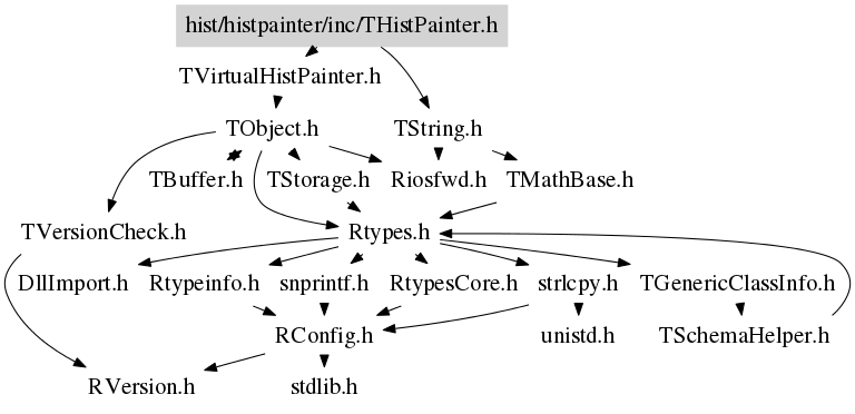

Function documentation
Compute the distance from the point px,py to a line.
Compute the closest distance of approach from point px,py to elements of an histogram. The distance is computed in pixels units.
Algorithm:
Currently, this simple model computes the distance from the mouse to the
histogram contour only.
Execute the actions corresponding to "event".
This function is called when a histogram is clicked with the locator at the pixel position px,py.
Get a contour (as a list of TGraphs) using the Delaunay triangulation.
Display the histogram info (bin number, contents, integral up to bin corresponding to cursor position px,py.
Return kTRUE if the cell ix, iy is inside one of the graphical cuts.
Return kTRUE if the point x,y is inside one of the graphical cuts.
Draw axis (2D case) of an histogram.
If drawGridOnly is TRUE, only the grid is painted (if needed). This allows to draw the grid and the axis separately. In THistPainter::Paint this feature is used to make sure that the grid is drawn in the background and the axis tick marks in the foreground of the pad.
Fill the matrix XARR YARR for Contour Plot.
Static function to paint special objects like vectors and matrices. This function is called via gROOT->ProcessLine to paint these objects without having a direct dependency of the graphics or histogramming system.
Control function to draw a TH2Poly bins' contours. option = "F" draw the bins as filled areas. option = "L" draw the bins as line. option = "P" draw the bins as markers.
Draw the histogram title
The title is drawn according to the title alignment returned by GetTitleAlign(). It is a 2 digits integer): hv
where "h" is the horizontal alignment and "v" is the vertical alignment.
- "h" can get the values 1 2 3 for left, center, and right
- "v" can get the values 1 2 3 for bottom, middle and top
Static function.
Convert Right Ascension, Declination to X,Y using an AITOFF projection. This procedure can be used to create an all-sky map in Galactic coordinates with an equal-area Aitoff projection. Output map coordinates are zero longitude centered. Also called Hammer-Aitoff projection (first presented by Ernst von Hammer in 1892)
source: GMT
code from Ernst-Jan Buis
Static function
Probably the most famous of the various map projections, the Mercator projection takes its name from Mercator who presented it in 1569. It is a cylindrical, conformal projection with no distortion along the equator. The Mercator projection has been used extensively for world maps in which the distortion towards the polar regions grows rather large, thus incorrectly giving the impression that, for example, Greenland is larger than South America. In reality, the latter is about eight times the size of Greenland. Also, the Former Soviet Union looks much bigger than Africa or South America. One may wonder whether this illusion has had any influence on U.S. foreign policy.' (Source: GMT) code from Ernst-Jan Buis
Static function code from Ernst-Jan Buis
Static function code from Ernst-Jan Buis
This function returns the best format to print the error value (e) knowing the parameter value (v) and the format (f) used to print it.
Show projection (specified by fShowProjection) of a TH3. The drawing option for the projection is in fShowOption.
First implementation; R.Brun
Full implementation: Tim Tran (timtran@jlab.org) April 2006