FourBinInstructional.py File Reference

Detailed Description

This example is a generalization of the on/off problem.

This example is a generalization of the on/off problem. It's a common setup for SUSY searches. Imagine that one has two variables "x" and "y" (eg. missing ET and SumET), see figure. The signal region has high values of both of these variables (top right). One can see low values of "x" or "y" acting as side-bands. If we just used "y" as a sideband, we would have the on/off problem.

• In the signal region we observe non events and expect s+b events.
• In the region with low values of "y" (bottom right) we observe noff events and expect tau*b events. Note the significance of tau. In the background only case:

tau ~ <expectation off> / <expectation on>

If tau is known, this model is sufficient, but often tau is not known exactly. So one can use low values of "x" as an additional constraint for tau. Note that this technique critically depends on the notion that the joint distribution for "x" and "y" can be factorized. Generally, these regions have many events, so it the ratio can be measured very precisely there. So we extend the model to describe the left two boxes... denoted with "bar".

• In the upper left we observe nonbar events and expect bbar events
• In the bottom left we observe noffbar events and expect tau bbar events Note again we have:

tau ~ <expectation off bar> / <expectation on bar>

One can further expand the model to account for the systematic associated to assuming the distribution of "x" and "y" factorizes (eg. that tau is the same for off/on and offbar/onbar). This can be done in several ways, but here we introduce an additional parameter rho, which so that one set of models will use tau and the other tau*rho. The choice is arbitrary, but it has consequences on the numerical stability of the algorithms. The "bar" measurements typically have more events (& smaller relative errors). If we choose

<expectation noffbar> = tau * rho * <expectation noonbar>

the product tau*rho will be known very precisely (~1/sqrt(bbar)) and the contour in those parameters will be narrow and have a non-trivial tau~1/rho shape. However, if we choose to put rho on the non/noff measurements (where the product will have an error ~1/sqrt(b)), the contours will be more amenable to numerical techniques. Thus, here we choose to define:

   tau := <expectation off bar> / (<expectation on bar>)
   rho := <expectation off> / (<expectation on> * tau)
 
^ y
|
|---------------------------+
|               |           |
|     nonbar    |    non    |
|      bbar     |    s+b    |
|               |           |
|---------------+-----------|
|               |           |
|    noffbar    |    noff   |
|    tau bbar   | tau b rho |
|               |           |
+-----------------------------> x

Left in this way, the problem is under-constrained. However, one may have some auxiliary measurement (usually based on Monte Carlo) to constrain rho. Let us call this auxiliary measurement that gives the nominal value of rho "rhonom". Thus, there is a 'constraint' term in the full model: P(rhonom | rho). In this case, we consider a Gaussian constraint with standard deviation sigma.

In the example, the initial values of the parameters are:

- s    = 40
- b    = 100
- tau  = 5
- bbar = 1000
- rho  = 1
(sigma for rho = 20%)

and in the toy dataset:

- non = 139
- noff = 528
- nonbar = 993
- noffbar = 4906
- rhonom = 1.27824

Note, the covariance matrix of the parameters has large off-diagonal terms. Clearly s,b are anti-correlated. Similarly, since noffbar >> nonbar, one would expect bbar,tau to be anti-correlated.

This can be seen below.

       GLOBAL      b    bbar   rho      s     tau
   b  0.96820   1.000  0.191 -0.942 -0.762 -0.209
bbar  0.91191   0.191  1.000  0.000 -0.146 -0.912
 rho  0.96348  -0.942  0.000  1.000  0.718 -0.000
   s  0.76250  -0.762 -0.146  0.718  1.000  0.160
 tau  0.92084  -0.209 -0.912 -0.000  0.160  1.000

Similarly, since tau*rho appears as a product, we expect rho,tau to be anti-correlated. When the error on rho is significantly larger than 1/sqrt(bbar), tau is essentially known and the correlation is minimal (tau mainly cares about bbar, and rho about b,s). In the alternate parametrization (bbar* tau * rho) the correlation coefficient for rho,tau is large (and negative).

The code below uses best-practices for RooFit & RooStats as of June 2010.

It proceeds as follows:

• create a workspace to hold the model
• use workspace factory to quickly create the terms of the model
• use workspace factory to define total model (a prod pdf)
• create a RooStats ModelConfig to specify observables, parameters of interest
• add to the ModelConfig a prior on the parameters for Bayesian techniques note, the pdf it is factorized for parameters of interest & nuisance params
• visualize the model
• write the workspace to a file
• use several of RooStats IntervalCalculators & compare results

[#0] WARNING:InputArguments -- The parameter 'sigma' with range [-inf, inf] of the RooGaussian 'mcCons' exceeds the safe range of (0, inf). Advise to limit its range.
[#1] INFO:ObjectHandling -- RooWorkspace::import(wspace) importing dataset modelData
[#1] INFO:InputArguments -- The deprecated RooFit::CloneData(1) option passed to createNLL() is ignored.
[#1] INFO:Fitting -- RooAbsPdf::fitTo(model) fixing normalization set for coefficient determination to observables in data
[#1] INFO:Fitting -- using CPU computation library compiled with -mavx2
[#0] PROGRESS:Minimization -- ProfileLikelihoodCalcultor::DoGLobalFit - find MLE 
[#1] INFO:Fitting -- RooAddition::defaultErrorLevel(nll_model_modelData) Summation contains a RooNLLVar, using its error level
[#1] INFO:Minimization -- RooAbsMinimizerFcn::setOptimizeConst: activating const optimization
[#0] PROGRESS:Minimization -- ProfileLikelihoodCalcultor::DoMinimizeNLL - using Minuit2 /  with strategy 1
[#1] INFO:Minimization -- 
  RooFitResult: minimized FCN value: 16.2872, estimated distance to minimum: 3.95421e-11
                covariance matrix quality: Full, accurate covariance matrix
                Status : MINIMIZE=0 
 
    Floating Parameter    FinalValue +/-  Error   
  --------------------  --------------------------
                     b    8.3599e+01 +/-  1.39e+01
                  bbar    9.9300e+02 +/-  3.15e+01
                   rho    1.2784e+00 +/-  1.99e-01
                     s    5.5401e+01 +/-  1.78e+01
                   tau    4.9406e+00 +/-  1.72e-01
 
[#1] INFO:Fitting -- RooAbsPdf::fitTo(model) fixing normalization set for coefficient determination to observables in data
[#1] INFO:Fitting -- RooAddition::defaultErrorLevel(nll_model_modelData) Summation contains a RooNLLVar, using its error level
[#1] INFO:Minimization -- RooAbsMinimizerFcn::setOptimizeConst: activating const optimization
Minuit2Minimizer: Minimize with max-calls 2500 convergence for edm < 1 strategy 1
Minuit2Minimizer : Valid minimum - status = 0
FVAL  = 16.2877177140194611
Edm   = 0.000501273030217960834
Nfcn  = 161
b    = 83.623   +/-  13.8829  (limited)
bbar    = 992.062  +/-  31.4883  (limited)
rho     = 1.27663  +/-  0.1986   (limited)
s    = 55.4234  +/-  17.8323  (limited)
tau     = 4.9456   +/-  0.171969 (limited)
[#1] INFO:Minimization -- RooAbsMinimizerFcn::setOptimizeConst: deactivating const optimization
[#1] INFO:Minimization -- RooProfileLL::evaluate(RooEvaluatorWrapper_Profile[s]) Creating instance of MINUIT
[#1] INFO:Fitting -- RooAddition::defaultErrorLevel(nll_model_modelData) Summation contains a RooNLLVar, using its error level
[#1] INFO:Minimization -- RooProfileLL::evaluate(RooEvaluatorWrapper_Profile[s]) determining minimum likelihood for current configurations w.r.t all observable
[#1] INFO:Minimization -- RooProfileLL::evaluate(RooEvaluatorWrapper_Profile[s]) minimum found at (s=55.3281)
.
[#1] INFO:Minimization -- RooProfileLL::evaluate(RooEvaluatorWrapper_Profile[s]) Creating instance of MINUIT
[#1] INFO:Fitting -- RooAddition::defaultErrorLevel(nll_model_modelData) Summation contains a RooNLLVar, using its error level
[#1] INFO:Minimization -- RooProfileLL::evaluate(RooEvaluatorWrapper_Profile[s]) determining minimum likelihood for current configurations w.r.t all observable
[#0] ERROR:InputArguments -- RooArgSet::checkForDup: ERROR argument with name s is already in this set
[#1] INFO:Minimization -- RooProfileLL::evaluate(RooEvaluatorWrapper_Profile[s]) minimum found at (s=55.3928)
..........................................................................................................................................................................................................Real time 0:00:01, CP time 1.390
Bayesian Calc. only supports on parameter of interest
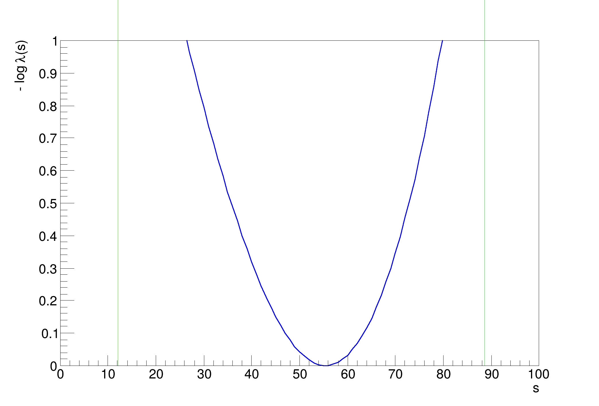
Profile Likelihood interval on s = [12.190172913897769, 88.68711754358463]

 
import ROOT
 
doBayesian = False
doFeldmanCousins = False
doMCMC = False
 
# let's time this challenging example
t = ROOT.TStopwatch()
t.Start()
 
# set RooFit random seed for reproducible results
ROOT.RooRandom.randomGenerator().SetSeed(4357)
 
# make model
wspace = ROOT.RooWorkspace("wspace")
wspace.factory("Poisson::on(non[0,1000], sum::splusb(s[40,0,100],b[100,0,300]))")
wspace.factory("Poisson::off(noff[0,5000], prod::taub(b,tau[5,3,7],rho[1,0,2]))")
wspace.factory("Poisson::onbar(nonbar[0,10000], bbar[1000,500,2000])")
wspace.factory("Poisson::offbar(noffbar[0,1000000], prod::lambdaoffbar(bbar, tau))")
wspace.factory("Gaussian::mcCons(rhonom[1.,0,2], rho, sigma[.2])")
wspace.factory("PROD::model(on,off,onbar,offbar,mcCons)")
wspace.defineSet("obs", "non,noff,nonbar,noffbar,rhonom")
 
wspace.factory("Uniform::prior_poi({s})")
wspace.factory("Uniform::prior_nuis({b,bbar,tau, rho})")
wspace.factory("PROD::prior(prior_poi,prior_nuis)")
 
# ----------------------------------
# Control some interesting variations
# define parameers of interest
# for 1-d plots
wspace.defineSet("poi", "s")
wspace.defineSet("nuis", "b,tau,rho,bbar")
 
# for 2-d plots to inspect correlations:
# wspace.defineSet("poi","s,rho")
 
# test simpler cases where parameters are known.
# wspace["tau"].setConstant()
# wspace["rho"].setConstant()
# wspace["b"].setConstant()
# wspace["bbar"].setConstant()
 
# inspect workspace
# wspace.Print()
 
# ----------------------------------------------------------
# Generate toy data
# generate toy data assuming current value of the parameters
# import into workspace.
# add Verbose() to see how it's being generated
data = wspace["model"].generate(wspace.set("obs"), 1)
# data.Print("v")
wspace.Import(data)
 
# ----------------------------------
# Now the statistical tests
# model config
modelConfig = ROOT.RooStats.ModelConfig("FourBins")
modelConfig.SetWorkspace(wspace)
modelConfig.SetPdf(wspace["model"])
modelConfig.SetPriorPdf(wspace["prior"])
modelConfig.SetParametersOfInterest(wspace.set("poi"))
modelConfig.SetNuisanceParameters(wspace.set("nuis"))
wspace.Import(modelConfig)
# wspace.writeToFile("FourBin.root")
 
# -------------------------------------------------
# If you want to see the covariance matrix uncomment
# wspace["model"].fitTo(data)
 
# use ProfileLikelihood
plc = ROOT.RooStats.ProfileLikelihoodCalculator(data, modelConfig)
plc.SetConfidenceLevel(0.95)
plInt = plc.GetInterval()
msglevel = ROOT.RooMsgService.instance().globalKillBelow()
ROOT.RooMsgService.instance().setGlobalKillBelow(ROOT.RooFit.FATAL)
plInt.LowerLimit(wspace["s"])  # get ugly print out of the way. Fix.
ROOT.RooMsgService.instance().setGlobalKillBelow(msglevel)
 
# use FeldmaCousins (takes ~20 min)
fc = ROOT.RooStats.FeldmanCousins(data, modelConfig)
fc.SetConfidenceLevel(0.95)
# number counting: dataset always has 1 entry with N events observed
fc.FluctuateNumDataEntries(False)
fc.UseAdaptiveSampling(True)
fc.SetNBins(40)
fcInt = ROOT.RooStats.PointSetInterval()
if doFeldmanCousins:  # takes 7 minutes
    fcInt = fc.GetInterval()
 
# use BayesianCalculator (only 1-d parameter of interest, slow for this problem)
bc = ROOT.RooStats.BayesianCalculator(data, modelConfig)
bc.SetConfidenceLevel(0.95)
bInt = ROOT.RooStats.SimpleInterval()
if doBayesian and len(wspace.set("poi")) == 1:
    bInt = bc.GetInterval()
else:
    print("Bayesian Calc. only supports on parameter of interest")
 
# use MCMCCalculator  (takes about 1 min)
# Want an efficient proposal function, so derive it from covariance
# matrix of fit
fit = wspace["model"].fitTo(data, Save=True)
ph = ROOT.RooStats.ProposalHelper()
ph.SetVariables(fit.floatParsFinal())
ph.SetCovMatrix(fit.covarianceMatrix())
ph.SetUpdateProposalParameters(ROOT.kTRUE)  # auto-create mean vars and add mappings
ph.SetCacheSize(100)
pf = ph.GetProposalFunction()
 
mc = ROOT.RooStats.MCMCCalculator(data, modelConfig)
mc.SetConfidenceLevel(0.95)
mc.SetProposalFunction(pf)
mc.SetNumBurnInSteps(500)  # first N steps to be ignored as burn-in
mc.SetNumIters(50000)
mc.SetLeftSideTailFraction(0.5)  # make a central interval
mcInt = ROOT.RooStats.MCMCInterval()
if doMCMC:
    mcInt = mc.GetInterval()
 
# ----------------------------------
# Make some plots
c1 = ROOT.gROOT.Get("c1")
if not c1:
    c1 = ROOT.TCanvas("c1")
 
if doBayesian and doMCMC:
    c1.Divide(3)
    c1.cd(1)
elif doBayesian or doMCMC:
    c1.Divide(2)
    c1.cd(1)
 
lrplot = ROOT.RooStats.LikelihoodIntervalPlot(plInt)
lrplot.Draw()
 
if doBayesian and len(wspace.set("poi")) == 1:
    c1.cd(2)
    # the plot takes a long time and print lots of error
    # using a scan it is better
    bc.SetScanOfPosterior(20)
    bplot = bc.GetPosteriorPlot()
    bplot.Draw()
 
if doMCMC:
    if doBayesian and len(wspace.set("poi")) == 1:
        c1.cd(3)
    else:
        c1.cd(2)
    mcPlot = ROOT.RooStats.MCMCIntervalPlot(mcInt)
    mcPlot.Draw()
 
# ----------------------------------
# query intervals
print(
    "Profile Likelihood interval on s = [{}, {}]".format(plInt.LowerLimit(wspace["s"]), plInt.UpperLimit(wspace["s"]))
)
# Profile Likelihood interval on s = [12.1902, 88.6871]
 
if doBayesian and len(wspace.set("poi")) == 1:
    print("Bayesian interval on s = [{}, {}]".format(bInt.LowerLimit(), bInt.UpperLimit()))
 
if doFeldmanCousins:
    print(
        "Feldman Cousins interval on s = [{}, {}]".format(fcInt.LowerLimit(wspace["s"]), fcInt.UpperLimit(wspace["s"]))
    )
    # Feldman Cousins interval on s = [18.75 +/- 2.45, 83.75 +/- 2.45]
 
if doMCMC:
    print("MCMC interval on s = [{}, {}]".format(mcInt.LowerLimit(wspace["s"]), mcInt.UpperLimit(wspace["s"])))
    # MCMC interval on s = [15.7628, 84.7266]
 
t.Stop()
t.Print()
 
c1.SaveAs("FourBinInstructional.png")
 
# TODO: The calculators have to be destructed first. Otherwise, we can get
# segmentation faults depending on the destruction order, which is random in
# Python. Probably the issue is that some object has a non-owning pointer to
# another object, which it uses in its destructor. This should be fixed either
# in the design of RooStats in C++, or with phythonizations.
del plc
del bc
del mc

Date

July 2022

Authors

Artem Busorgin, Kyle Cranmer and Tanja Rommerskirchen (C++ version)

Definition in file FourBinInstructional.py.