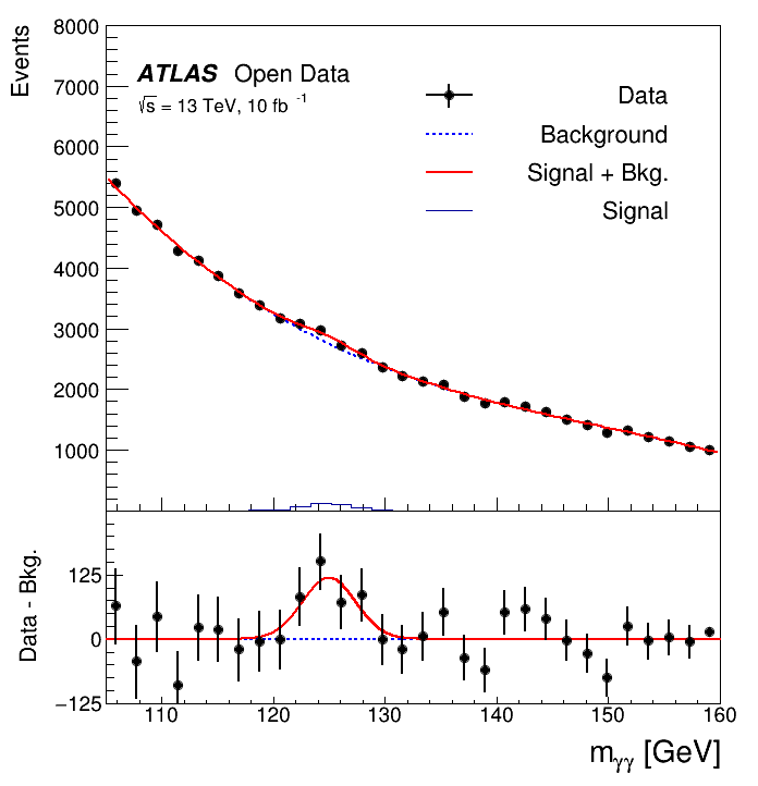
The data was taken with the ATLAS detector during 2016 at a center-of-mass energy of 13 TeV. Although the Higgs to two photons decay is very rare, the contribution of the Higgs can be seen as a narrow peak around 125 GeV because of the excellent reconstruction and identification efficiency of photons at the ATLAS experiment.
The analysis is translated to a RDataFrame workflow processing 1.7 GB of simulated events and data.
import ROOT
import os
ROOT.ROOT.EnableImplicitMT()
path = "root://eospublic.cern.ch//eos/opendata/atlas/OutreachDatasets/2020-01-22"
df = {}
df[
"data"] =
ROOT.RDataFrame(
"mini", (os.path.join(path,
"GamGam/Data/data_{}.GamGam.root".format(x))
for x
in (
"A",
"B",
"C",
"D")))
df[
"ggH"] =
ROOT.RDataFrame(
"mini", os.path.join(path,
"GamGam/MC/mc_343981.ggH125_gamgam.GamGam.root"))
df[
"VBF"] =
ROOT.RDataFrame(
"mini", os.path.join(path,
"GamGam/MC/mc_345041.VBFH125_gamgam.GamGam.root"))
processes = list(df.keys())
for p in ["ggH", "VBF"]:
df[p] = df[p].Define("weight",
"scaleFactor_PHOTON * scaleFactor_PhotonTRIGGER * scaleFactor_PILEUP * mcWeight");
df["data"] = df["data"].Define("weight", "1.0")
for p in processes:
df[p] = df[p].Define("goodphotons", "photon_isTightID && (photon_pt > 25000) && (abs(photon_eta) < 2.37) && ((abs(photon_eta) < 1.37) || (abs(photon_eta) > 1.52))")\
.
Filter(
"Sum(goodphotons) == 2")
df[p] = df[p].
Filter(
"Sum(photon_ptcone30[goodphotons] / photon_pt[goodphotons] < 0.065) == 2")\
.
Filter(
"Sum(photon_etcone20[goodphotons] / photon_pt[goodphotons] < 0.065) == 2")
ROOT.gInterpreter.Declare(
"""
using Vec_t = const ROOT::VecOps::RVec<float>;
float ComputeInvariantMass(Vec_t& pt, Vec_t& eta, Vec_t& phi, Vec_t& e) {
ROOT::Math::PtEtaPhiEVector p1(pt[0], eta[0], phi[0], e[0]);
ROOT::Math::PtEtaPhiEVector p2(pt[1], eta[1], phi[1], e[1]);
return (p1 + p2).mass() / 1000.0;
}
""")
# Define a new column with the invariant mass and perform final event selection
hists = {}
for p in processes:
df[p] = df[p].Define("m_yy", "ComputeInvariantMass(photon_pt[goodphotons], photon_eta[goodphotons], photon_phi[goodphotons], photon_E[goodphotons])")
df[p] = df[p].
Filter(
"photon_pt[goodphotons][0] / 1000.0 / m_yy > 0.35")\
.
Filter(
"photon_pt[goodphotons][1] / 1000.0 / m_yy > 0.25")\
.
Filter(
"m_yy > 105 && m_yy < 160")
hists[p] = df[p].Histo1D(
ROOT.RDF.TH1DModel(p,
"Diphoton invariant mass; m_{#gamma#gamma} [GeV];Events", 30, 105, 160),
"m_yy", "weight")
ggh = hists["ggH"].GetValue()
vbf = hists["VBF"].GetValue()
data = hists["data"].GetValue()
ROOT.gROOT.SetStyle("ATLAS")
c = ROOT.TCanvas("c", "", 700, 750)
upper_pad = ROOT.TPad("upper_pad", "", 0, 0.35, 1, 1)
lower_pad = ROOT.TPad("lower_pad", "", 0, 0, 1, 0.35)
for p in [upper_pad, lower_pad]:
p.SetLeftMargin(0.14)
p.SetRightMargin(0.05)
p.SetTickx(False)
p.SetTicky(False)
upper_pad.SetBottomMargin(0)
lower_pad.SetTopMargin(0)
lower_pad.SetBottomMargin(0.3)
upper_pad.Draw()
lower_pad.Draw()
upper_pad.cd()
fit = ROOT.TF1("fit", "([0]+[1]*x+[2]*x^2+[3]*x^3)+[4]*exp(-0.5*((x-[5])/[6])^2)", 105, 160)
fit.FixParameter(5, 125.0)
fit.FixParameter(4, 119.1)
fit.FixParameter(6, 2.39)
fit.SetLineColor(2)
fit.SetLineStyle(1)
fit.SetLineWidth(2)
data.Fit("fit", "", "E SAME", 105, 160)
fit.Draw("SAME")
bkg = ROOT.TF1("bkg", "([0]+[1]*x+[2]*x^2+[3]*x^3)", 105, 160)
for i in range(4):
bkg.SetParameter(i, fit.GetParameter(i))
bkg.SetLineColor(4)
bkg.SetLineStyle(2)
bkg.SetLineWidth(2)
bkg.Draw("SAME")
data.SetMarkerStyle(20)
data.SetMarkerSize(1.2)
data.SetLineWidth(2)
data.SetLineColor(ROOT.kBlack)
data.Draw("E SAME")
data.SetMinimum(1e-3)
data.SetMaximum(8e3)
data.GetYaxis().SetLabelSize(0.045)
data.GetYaxis().SetTitleSize(0.05)
data.SetStats(0)
data.SetTitle("")
lumi = 10064.0
ggh.Scale(lumi * 0.102 / 55922617.6297)
vbf.Scale(lumi * 0.008518764 / 3441426.13711)
higgs = ggh.Clone()
higgs.Add(vbf)
higgs.Draw("HIST SAME")
lower_pad.cd()
ratiobkg = ROOT.TF1("zero", "0", 105, 160)
ratiobkg.SetLineColor(4)
ratiobkg.SetLineStyle(2)
ratiobkg.SetLineWidth(2)
ratiobkg.SetMinimum(-125)
ratiobkg.SetMaximum(250)
ratiobkg.GetXaxis().SetLabelSize(0.08)
ratiobkg.GetXaxis().SetTitleSize(0.12)
ratiobkg.GetXaxis().SetTitleOffset(1.0)
ratiobkg.GetYaxis().SetLabelSize(0.08)
ratiobkg.GetYaxis().SetTitleSize(0.09)
ratiobkg.GetYaxis().SetTitle("Data - Bkg.")
ratiobkg.GetYaxis().CenterTitle()
ratiobkg.GetYaxis().SetTitleOffset(0.7)
ratiobkg.GetYaxis().SetNdivisions(503, False)
ratiobkg.GetYaxis().ChangeLabel(-1, -1, 0)
ratiobkg.GetXaxis().SetTitle("m_{#gamma#gamma} [GeV]")
ratiobkg.Draw()
ratiosig = ROOT.TH1F("ratiosig", "ratiosig", 5500, 105, 160)
ratiosig.Eval(fit)
ratiosig.SetLineColor(2)
ratiosig.SetLineStyle(1)
ratiosig.SetLineWidth(2)
ratiosig.Add(bkg, -1)
ratiosig.Draw("SAME")
ratiodata = data.Clone()
ratiodata.Add(bkg, -1)
ratiodata.Draw("E SAME")
for i in range(1, data.GetNbinsX()):
ratiodata.SetBinError(i, data.GetBinError(i))
upper_pad.cd()
legend = ROOT.TLegend(0.55, 0.55, 0.89, 0.85)
legend.SetTextFont(42)
legend.SetFillStyle(0)
legend.SetBorderSize(0)
legend.SetTextSize(0.05)
legend.SetTextAlign(32)
legend.AddEntry(data, "Data" ,"lep")
legend.AddEntry(bkg, "Background", "l")
legend.AddEntry(fit, "Signal + Bkg.", "l")
legend.AddEntry(higgs, "Signal", "l")
legend.Draw("SAME")
text = ROOT.TLatex()
text.SetNDC()
text.SetTextFont(72)
text.SetTextSize(0.05)
text.DrawLatex(0.18, 0.84, "ATLAS")
text.SetTextFont(42)
text.DrawLatex(0.18 + 0.13, 0.84, "Open Data")
text.SetTextSize(0.04)
text.DrawLatex(0.18, 0.78, "#sqrt{s} = 13 TeV, 10 fb^{-1}");
c.SaveAs("HiggsToTwoPhotons.pdf");
ROOT's RDataFrame offers a high level interface for analyses of data stored in TTrees,...
RVec< T > Filter(const RVec< T > &v, F &&f)
Create a new collection with the elements passing the filter expressed by the predicate.
A struct which stores the parameters of a TH1D.