rf615_simulation_based_inference.py File Reference

Detailed Description

Use Simulation Based Inference (SBI) in RooFit.

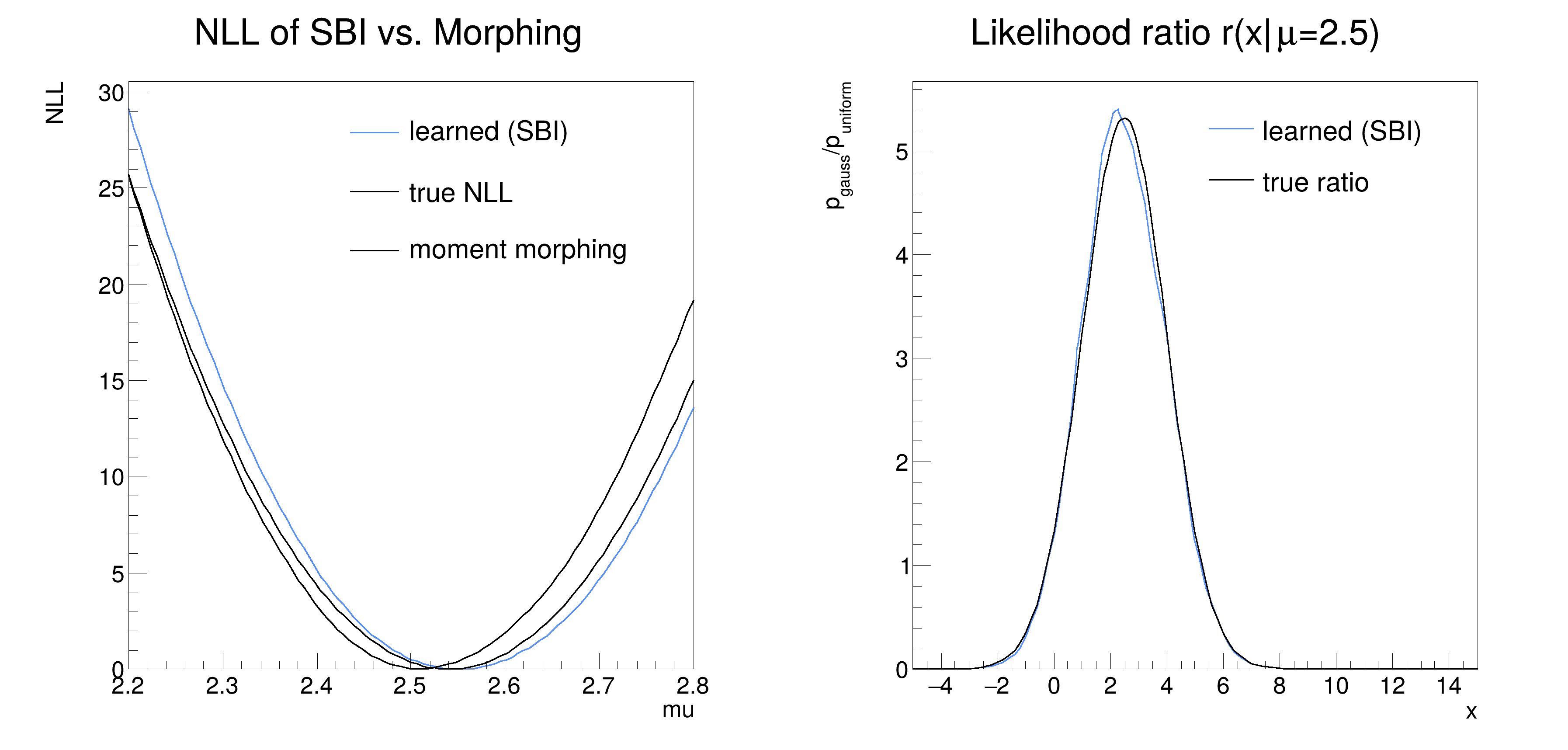
This tutorial shows how to use SBI in ROOT. As reference distribution we choose a simple uniform distribution. The target distribution is chosen to be gaussian with different mean values. The classifier is trained to discriminate between the reference and target distribution. We see how the neural networks generalize to unknown mean values.

We compare the approach of using the likelihood ratio trick to morphing.

An introduction of SBI can be found in https://arxiv.org/pdf/2010.06439.

A short recap: The idea of SBI is to fit a surrogate model to the data, in order to really learn the likelihood function instead of calculating it. Therefore, a classifier is trained to discriminate between samples from a target distribution (here the Gaussian) $$x\sim p(x|\theta)$$ and a reference distribution (here the Uniform) $$x\sim p_{ref}(x|\theta)$$.

The output of the classifier $$\hat{s}(\theta)$$ is a monotonic function of the likelihood ration and can be turned into an estimate of the likelihood ratio via $$\hat{r}(\theta)=\frac{1-\hat{s}(\theta)}{\hat{s}(\theta)}.$$ This is called the likelihood ratio trick.

In the end we compare the negative logarithmic likelihoods of the learned, morphed and analytical likelihood with minuit and as a plot.

 
import ROOT
import numpy as np
from sklearn.neural_network import MLPClassifier
 
# The samples used for training the classifier in this tutorial / rescale for more accuracy
n_samples = 10000
 
# Kills warning messages
ROOT.RooMsgService.instance().setGlobalKillBelow(ROOT.RooFit.WARNING)
 
 
# Morphing as a baseline
def morphing(setting):
 
    # Define binning for morphing
    grid = ROOT.RooMomentMorphFuncND.Grid(ROOT.RooBinning(4, 0.0, 4.0))
    x_var.setBins(50)
 
    # Number of 'sampled' gaussians, if you change it, adjust the binning properly
    n_grid = 5
 
    for i in range(n_grid):
        # Define the sampled gausians
        mu_help = ROOT.RooRealVar(f"mu{i}", f"mu{i}", i)
        help = ROOT.RooGaussian(f"g{i}", f"g{i}", x_var, mu_help, sigma)
        workspace.Import(help, Silence=True)
 
        # Fill the histograms
        hist = workspace[f"g{i}"].generateBinned([x_var], n_samples)
 
        # Make sure that every bin is filled and we don't get zero probability
        for i_bin in range(hist.numEntries()):
            hist.add(hist.get(i_bin), 1.0)
 
        # Add the pdf to the workspace
        workspace.Import(ROOT.RooHistPdf(f"histpdf{i}", f"histpdf{i}", [x_var], hist, 1), Silence=True)
 
        # Add the pdf to the grid
        grid.addPdf(workspace[f"histpdf{i}"], i)
 
    # Create the morphing and add it to the workspace
    morph_func = ROOT.RooMomentMorphFuncND("morph_func", "morph_func", [mu_var], [x_var], grid, setting)
    morph = ROOT.RooWrapperPdf("morph", "morph", morph_func, True)
    workspace.Import(morph, Silence=True)
 
    # Uncomment to see input plots for the first dimension (you might need to increase the morphed samples)
    # f1 = x_var.frame(Title="linear morphing;x;pdf", Range=(-4, 8))
    # for i in range(n_grid):
    # workspace[f"histpdf{i}"].plotOn(f1)
    # workspace["morph"].plotOn(f1, LineColor="r")
    # c0 = ROOT.TCanvas()
    # f1.Draw()
    # input() # Wait for user input to proceed
 
 
# Class used in this case to demonstrate the use of SBI in Root
class SBI:
    # Initializing the class SBI
    def __init__(self, workspace):
        # Choose the hyperparameters for training the neural network
        self.classifier = MLPClassifier(hidden_layer_sizes=(20, 20), max_iter=1000, random_state=42)
        self.data_model = None
        self.data_ref = None
        self.X_train = None
        self.y_train = None
        self.workspace = workspace
 
    # Defining the target / training data for different values of mean value mu
    def model_data(self, model, x, mu, n_samples):
        ws = self.workspace
        data_test_model = []
        samples_gaussian = ws[model].generate([ws[x], ws[mu]], n_samples).to_numpy()
        self._training_mus = samples_gaussian[mu]
        data_test_model.extend(samples_gaussian[x])
 
        self.data_model = np.array(data_test_model).reshape(-1, 1)
 
    # Generating samples for the reference distribution
    def reference_data(self, model, x, n_samples):
        ws = self.workspace
        # Ensuring the normalization with generating as many reference data as target data
        samples_uniform = ws[model].generate(ws[x], n_samples)
        data_reference_model = np.array(
            [samples_uniform.get(i).getRealValue("x") for i in range(samples_uniform.numEntries())]
        )
        self.data_ref = data_reference_model.reshape(-1, 1)
 
    # Bringing the data in the right format for training
    def preprocessing(self):
        thetas_model = self._training_mus.reshape(-1, 1)
        thetas_reference = self._training_mus.reshape(-1, 1)
        thetas = np.concatenate((thetas_model, thetas_reference), axis=0)
        X = np.concatenate([self.data_model, self.data_ref])
        self.y_train = np.concatenate([np.ones(len(self.data_model)), np.zeros(len(self.data_ref))])
        self.X_train = np.concatenate([X, thetas], axis=1)
 
    # Train the classifier
    def train_classifier(self):
        self.classifier.fit(self.X_train, self.y_train)
 
 
# Setting the training and toy data samples; the factor 5 to enable a fair comparison to morphing
n_samples_train = n_samples * 5
 
 
# Define the "observed" data in a workspace
def build_ws(mu_observed, sigma):
    # using a workspace for easier processing inside the class
    ws = ROOT.RooWorkspace()
    ws.factory(f"Gaussian::gauss(x[-5,15], mu[0,4], {sigma})")
    ws.factory("Uniform::uniform(x)")
    ws["mu"].setVal(mu_observed)
    ws.Print("v")
    obs_data = ws["gauss"].generate(ws["x"], 1000)
    obs_data.SetName("obs_data")
    ws.Import(obs_data, Silence=True)
 
    return ws
 
 
# The "observed" data
mu_observed = 2.5
sigma = 1.5
workspace = build_ws(mu_observed, sigma)
x_var = workspace["x"]
mu_var = workspace["mu"]
gauss = workspace["gauss"]
uniform = workspace["uniform"]
obs_data = workspace["obs_data"]
 
# Training the model
model = SBI(workspace)
model.model_data("gauss", "x", "mu", n_samples_train)
model.reference_data("uniform", "x", n_samples_train)
model.preprocessing()
model.train_classifier()
sbi_model = model
 
 
# Compute the likelihood ratio of the classifier for analysis purposes
def learned_likelihood_ratio(x, mu):
    n = max(len(x), len(mu))
    X = np.zeros((n, 2))
    X[:, 0] = x
    X[:, 1] = mu
    prob = sbi_model.classifier.predict_proba(X)[:, 1]
    return prob / (1 - prob)
 
 
# Compute the learned likelihood ratio
llhr_learned = ROOT.RooFit.bindFunction("MyBinFunc", learned_likelihood_ratio, x_var, mu_var)
 
# Compute the real likelihood ratio
llhr_calc = ROOT.RooFormulaVar("llhr_calc", "x[0] / x[1]", [gauss, uniform])
 
# Create the exact negative log likelihood functions for Gaussian model
nll_gauss = gauss.createNLL(obs_data)
ROOT.SetOwnership(nll_gauss, True)
 
# Create the learned pdf and NLL sum based on the learned likelihood ratio
pdf_learned = ROOT.RooWrapperPdf("learned_pdf", "learned_pdf", llhr_learned, True)
 
nllr_learned = pdf_learned.createNLL(obs_data)
ROOT.SetOwnership(nllr_learned, True)
 
# Compute the morphed nll
morphing(ROOT.RooMomentMorphFuncND.Linear)
nll_morph = workspace["morph"].createNLL(obs_data)
ROOT.SetOwnership(nll_morph, True)
 
# Plot the negative logarithmic summed likelihood
frame1 = mu_var.frame(Title="NLL of SBI vs. Morphing;mu;NLL", Range=(2.2, 2.8))
nllr_learned.plotOn(frame1, LineColor="kP6Blue", ShiftToZero=True, Name="learned")
nll_gauss.plotOn(frame1, LineColor="kP6Blue+1", ShiftToZero=True, Name="gauss")
ROOT.RooAbsReal.setEvalErrorLoggingMode("Ignore")  # Silence some warnings
nll_morph.plotOn(frame1, LineColor="kP6Blue+2", ShiftToZero=True, Name="morphed")
ROOT.RooAbsReal.setEvalErrorLoggingMode("PrintErrors")
 
# Plot the likelihood functions
frame2 = x_var.frame(Title="Likelihood ratio r(x|#mu=2.5);x;p_{gauss}/p_{uniform}")
llhr_learned.plotOn(frame2, LineColor="kP6Blue", Name="learned_ratio")
llhr_calc.plotOn(frame2, LineColor="kP6Blue+1", Name="exact")
 
# Write the plots into one canvas to show, or into separate canvases for saving.
single_canvas = True
 
c = ROOT.TCanvas("", "", 1200 if single_canvas else 600, 600)
if single_canvas:
    c.Divide(2)
    c.cd(1)
    ROOT.gPad.SetLeftMargin(0.15)
    frame1.GetYaxis().SetTitleOffset(1.8)
frame1.Draw()
 
legend1 = ROOT.TLegend(0.43, 0.63, 0.8, 0.87)
legend1.SetFillColor(ROOT.kWhite)
legend1.SetLineColor(ROOT.kWhite)
legend1.SetTextSize(0.04)
legend1.AddEntry("learned", "learned (SBI)", "L")
legend1.AddEntry("gauss", "true NLL", "L")
legend1.AddEntry("morphed", "moment morphing", "L")
legend1.Draw()
 
if single_canvas:
    c.cd(2)
    ROOT.gPad.SetLeftMargin(0.15)
    frame2.GetYaxis().SetTitleOffset(1.8)
else:
    c.SaveAs("rf615_plot_1.png")
    c = ROOT.TCanvas("", "", 600, 600)
 
frame2.Draw()
 
legend2 = ROOT.TLegend(0.53, 0.73, 0.87, 0.87)
legend2.SetFillColor(ROOT.kWhite)
legend2.SetLineColor(ROOT.kWhite)
legend2.SetTextSize(0.04)
legend2.AddEntry("learned_ratio", "learned (SBI)", "L")
legend2.AddEntry("exact", "true ratio", "L")
legend2.Draw()
 
if not single_canvas:
    c.SaveAs("rf615_plot_2.png")
 
# Compute the minimum via minuit and display the results
for nll in [nll_gauss, nllr_learned, nll_morph]:
    minimizer = ROOT.RooMinimizer(nll)
    minimizer.setErrorLevel(0.5)  # Adjust the error level in the minimization to work with likelihoods
    minimizer.setPrintLevel(-1)
    minimizer.minimize("Minuit2")
    result = minimizer.save()
    ROOT.SetOwnership(result, True)
    result.Print()
 
del nll_morph
del nllr_learned
del nll_gauss
del workspace
 
import sys
 
# Hack to bypass ClearProxiedObjects()
del sys.modules["libROOTPythonizations"]

 
RooWorkspace()  contents
 
variables
---------
(mu,x)
 
p.d.f.s
-------
RooGaussian::gauss[ x=x mean=mu sigma=1.5 ] = 0.249352
RooUniform::uniform[ x=(x) ] = 1
 
 
  RooFitResult: minimized FCN value: 1862.97, estimated distance to minimum: 2.32702e-05
                covariance matrix quality: Full, accurate covariance matrix
                Status : MINIMIZE=0 
 
    Floating Parameter    FinalValue +/-  Error   
  --------------------  --------------------------
                    mu    2.5399e+00 +/-  4.74e-02
 
 
  RooFitResult: minimized FCN value: -1126.14, estimated distance to minimum: 4.23342e-05
                covariance matrix quality: Full, accurate covariance matrix
                Status : MINIMIZE=0 
 
    Floating Parameter    FinalValue +/-  Error   
  --------------------  --------------------------
                    mu    2.5511e+00 +/-  7.15e-02
 
 
  RooFitResult: minimized FCN value: 1864.58, estimated distance to minimum: 1.67611e-06
                covariance matrix quality: Full, accurate covariance matrix
                Status : MINIMIZE=0 
 
    Floating Parameter    FinalValue +/-  Error   
  --------------------  --------------------------
                    mu    2.5108e+00 +/-  4.09e-02
 

Date

July 2024

Author

Robin Syring

Definition in file rf615_simulation_based_inference.py.