[#1] INFO:Fitting -- RooAbsPdf::fitTo(model) fixing normalization set for coefficient determination to observables in data
[#1] INFO:Fitting -- using generic CPU library compiled with no vectorizations
[#1] INFO:Fitting -- Creation of NLL object took 938.355 μs
[#1] INFO:Fitting -- RooAddition::defaultErrorLevel(nll_model_genData) Summation contains a RooNLLVar, using its error level
[#1] INFO:Minimization -- [fitFCN] No discrete parameters, performing continuous minimization only
[#0] WARNING:InputArguments -- RooAbsReal::plotOn(model) WARNING: argument CurveNameSuffix is duplicated
[#0] WARNING:InputArguments -- RooAbsReal::plotOn(model) WARNING: argument CurveNameSuffix is duplicated
[#0] WARNING:InputArguments -- RooAbsReal::plotOn(model) WARNING: argument CurveNameSuffix is duplicated
[#0] WARNING:InputArguments -- RooAbsReal::plotOn(model) WARNING: argument CurveNameSuffix is duplicated
[#0] WARNING:InputArguments -- RooAbsReal::plotOn(model) WARNING: argument CurveNameSuffix is duplicated
[#0] WARNING:InputArguments -- RooAbsReal::plotOn(model) WARNING: argument CurveNameSuffix is duplicated
[#0] WARNING:InputArguments -- RooAbsReal::plotOn(model) WARNING: argument CurveNameSuffix is duplicated
[#0] WARNING:InputArguments -- RooAbsReal::plotOn(model) WARNING: argument CurveNameSuffix is duplicated
[#0] WARNING:InputArguments -- RooAbsReal::plotOn(model) WARNING: argument CurveNameSuffix is duplicated
[#0] WARNING:InputArguments -- RooAbsReal::plotOn(model) WARNING: argument CurveNameSuffix is duplicated
[#0] WARNING:InputArguments -- RooAbsReal::plotOn(model) WARNING: argument CurveNameSuffix is duplicated
[#0] WARNING:InputArguments -- RooAbsReal::plotOn(model) WARNING: argument CurveNameSuffix is duplicated
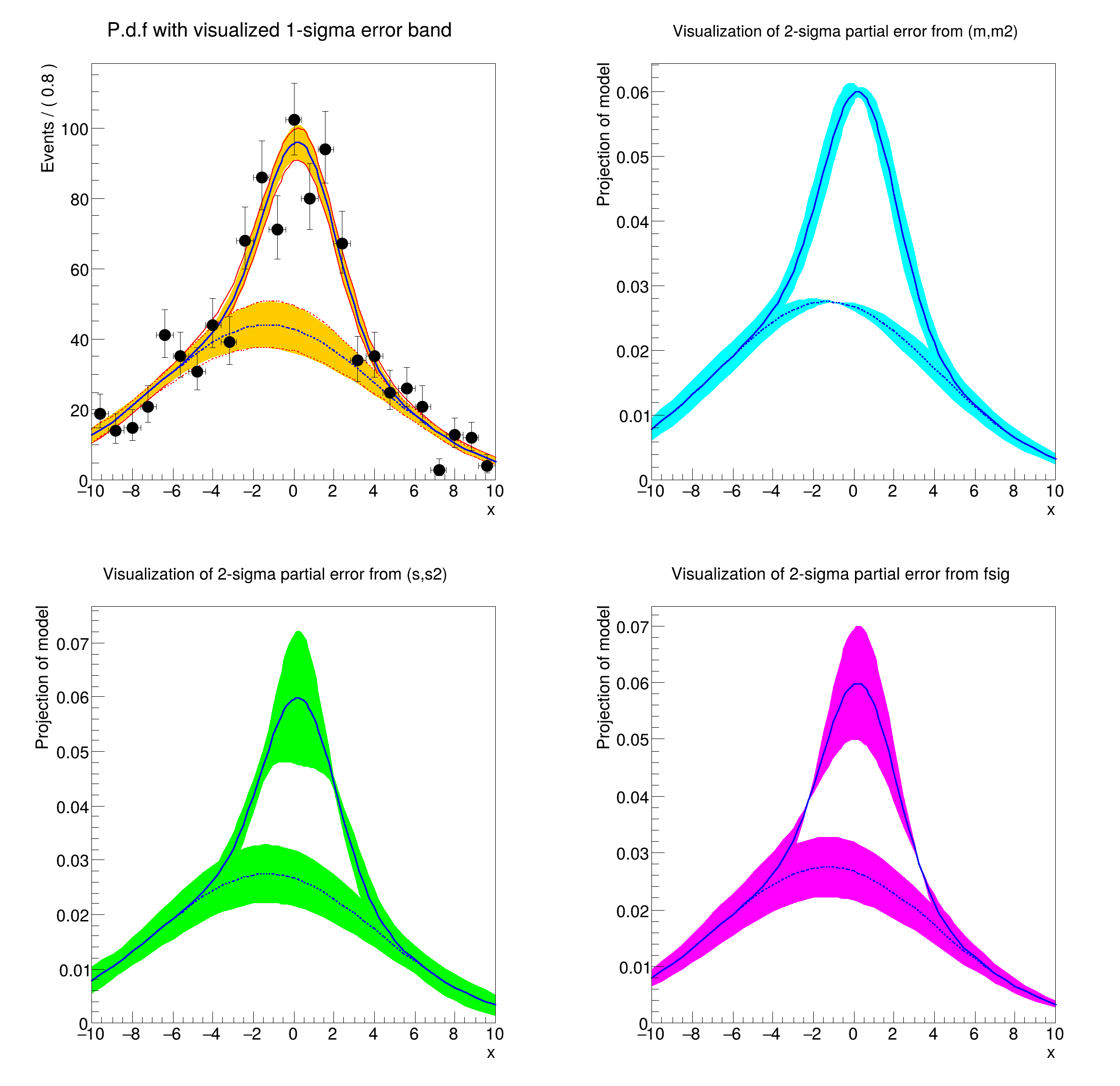
[#1] INFO:Plotting -- RooAbsReal::plotOn(model) INFO: visualizing 1-sigma uncertainties in parameters (m,s,fsig,m2,s2) from fit result fitresult_model_genData using 315 samplings.
[#0] WARNING:InputArguments -- RooAbsReal::plotOn(model) WARNING: argument CurveNameSuffix is duplicated
[#0] WARNING:InputArguments -- RooAbsReal::plotOn(model) WARNING: argument CurveNameSuffix is duplicated
[#0] WARNING:InputArguments -- RooAbsReal::plotOn(model) WARNING: argument CurveNameSuffix is duplicated
[#0] WARNING:InputArguments -- RooAbsReal::plotOn(model) WARNING: argument CurveNameSuffix is duplicated
[#0] WARNING:InputArguments -- RooAbsReal::plotOn(model) WARNING: argument CurveNameSuffix is duplicated
[#0] WARNING:InputArguments -- RooAbsReal::plotOn(model) WARNING: argument CurveNameSuffix is duplicated
[#0] WARNING:InputArguments -- RooAbsReal::plotOn(model) WARNING: argument CurveNameSuffix is duplicated
[#0] WARNING:InputArguments -- RooAbsReal::plotOn(model) WARNING: argument CurveNameSuffix is duplicated
[#0] WARNING:InputArguments -- RooAbsReal::plotOn(model) WARNING: argument CurveNameSuffix is duplicated
[#0] WARNING:InputArguments -- RooAbsReal::plotOn(model) WARNING: argument CurveNameSuffix is duplicated
[#0] WARNING:InputArguments -- RooAbsReal::plotOn(model) WARNING: argument CurveNameSuffix is duplicated
[#0] WARNING:InputArguments -- RooAbsReal::plotOn(model) WARNING: argument CurveNameSuffix is duplicated
[#0] WARNING:InputArguments -- RooAbsReal::plotOn(model) WARNING: argument CurveNameSuffix is duplicated
[#0] WARNING:InputArguments -- RooAbsReal::plotOn(model) WARNING: argument CurveNameSuffix is duplicated
[#0] WARNING:InputArguments -- RooAbsReal::plotOn(model) WARNING: argument CurveNameSuffix is duplicated
[#0] WARNING:InputArguments -- RooAbsReal::plotOn(model) WARNING: argument CurveNameSuffix is duplicated
[#0] WARNING:InputArguments -- RooAbsReal::plotOn(model) WARNING: argument CurveNameSuffix is duplicated
[#0] WARNING:InputArguments -- RooAbsReal::plotOn(model) WARNING: argument CurveNameSuffix is duplicated
[#0] WARNING:InputArguments -- RooAbsReal::plotOn(model) WARNING: argument CurveNameSuffix is duplicated
[#0] WARNING:InputArguments -- RooAbsReal::plotOn(model) WARNING: argument CurveNameSuffix is duplicated
[#0] WARNING:InputArguments -- RooAbsReal::plotOn(model) WARNING: argument CurveNameSuffix is duplicated
[#0] WARNING:InputArguments -- RooAbsReal::plotOn(model) WARNING: argument CurveNameSuffix is duplicated
[#0] WARNING:InputArguments -- RooAbsReal::plotOn(model) WARNING: argument CurveNameSuffix is duplicated
[#0] WARNING:InputArguments -- RooAbsReal::plotOn(model) WARNING: argument CurveNameSuffix is duplicated
[#0] WARNING:InputArguments -- RooAbsReal::plotOn(model) WARNING: argument CurveNameSuffix is duplicated
[#0] WARNING:InputArguments -- RooAbsReal::plotOn(model) WARNING: argument CurveNameSuffix is duplicated
[#0] WARNING:InputArguments -- RooAbsReal::plotOn(model) WARNING: argument CurveNameSuffix is duplicated
[#0] WARNING:InputArguments -- RooAbsReal::plotOn(model) WARNING: argument CurveNameSuffix is duplicated
[#0] WARNING:InputArguments -- RooAbsReal::plotOn(model) WARNING: argument CurveNameSuffix is duplicated
[#0] WARNING:InputArguments -- RooAbsReal::plotOn(model) WARNING: argument CurveNameSuffix is duplicated
[#0] WARNING:InputArguments -- RooAbsReal::plotOn(model) WARNING: argument CurveNameSuffix is duplicated
[#0] WARNING:InputArguments -- RooAbsReal::plotOn(model) WARNING: argument CurveNameSuffix is duplicated
[#0] WARNING:InputArguments -- RooAbsReal::plotOn(model) WARNING: argument CurveNameSuffix is duplicated
[#0] WARNING:InputArguments -- RooAbsReal::plotOn(model) WARNING: argument CurveNameSuffix is duplicated
[#0] WARNING:InputArguments -- RooAbsReal::plotOn(model) WARNING: argument CurveNameSuffix is duplicated
[#0] WARNING:InputArguments -- RooAbsReal::plotOn(model) WARNING: argument CurveNameSuffix is duplicated
[#0] WARNING:InputArguments -- RooAbsReal::plotOn(model) WARNING: argument CurveNameSuffix is duplicated
[#0] WARNING:InputArguments -- RooAbsReal::plotOn(model) WARNING: argument CurveNameSuffix is duplicated
[#0] WARNING:InputArguments -- RooAbsReal::plotOn(model) WARNING: argument CurveNameSuffix is duplicated
[#0] WARNING:InputArguments -- RooAbsReal::plotOn(model) WARNING: argument CurveNameSuffix is duplicated
[#0] WARNING:InputArguments -- RooAbsReal::plotOn(model) WARNING: argument CurveNameSuffix is duplicated
[#0] WARNING:InputArguments -- RooAbsReal::plotOn(model) WARNING: argument CurveNameSuffix is duplicated
[#0] WARNING:InputArguments -- RooAbsReal::plotOn(model) WARNING: argument CurveNameSuffix is duplicated
[#0] WARNING:InputArguments -- RooAbsReal::plotOn(model) WARNING: argument CurveNameSuffix is duplicated
[#0] WARNING:InputArguments -- RooAbsReal::plotOn(model) WARNING: argument CurveNameSuffix is duplicated
[#0] WARNING:InputArguments -- RooAbsReal::plotOn(model) WARNING: argument CurveNameSuffix is duplicated
[#0] WARNING:InputArguments -- RooAbsReal::plotOn(model) WARNING: argument CurveNameSuffix is duplicated
[#0] WARNING:InputArguments -- RooAbsReal::plotOn(model) WARNING: argument CurveNameSuffix is duplicated
[#0] WARNING:InputArguments -- RooAbsReal::plotOn(model) WARNING: argument CurveNameSuffix is duplicated
[#0] WARNING:InputArguments -- RooAbsReal::plotOn(model) WARNING: argument CurveNameSuffix is duplicated
[#0] WARNING:InputArguments -- RooAbsReal::plotOn(model) WARNING: argument CurveNameSuffix is duplicated
[#0] WARNING:InputArguments -- RooAbsReal::plotOn(model) WARNING: argument CurveNameSuffix is duplicated
[#0] WARNING:InputArguments -- RooAbsReal::plotOn(model) WARNING: argument CurveNameSuffix is duplicated
[#0] WARNING:InputArguments -- RooAbsReal::plotOn(model) WARNING: argument CurveNameSuffix is duplicated
[#0] WARNING:InputArguments -- RooAbsReal::plotOn(model) WARNING: argument CurveNameSuffix is duplicated
[#0] WARNING:InputArguments -- RooAbsReal::plotOn(model) WARNING: argument CurveNameSuffix is duplicated
[#0] WARNING:InputArguments -- RooAbsReal::plotOn(model) WARNING: argument CurveNameSuffix is duplicated
[#0] WARNING:InputArguments -- RooAbsReal::plotOn(model) WARNING: argument CurveNameSuffix is duplicated
[#0] WARNING:InputArguments -- RooAbsReal::plotOn(model) WARNING: argument CurveNameSuffix is duplicated
[#0] WARNING:InputArguments -- RooAbsReal::plotOn(model) WARNING: argument CurveNameSuffix is duplicated
[#0] WARNING:InputArguments -- RooAbsReal::plotOn(model) WARNING: argument CurveNameSuffix is duplicated
[#0] WARNING:InputArguments -- RooAbsReal::plotOn(model) WARNING: argument CurveNameSuffix is duplicated
[#0] WARNING:InputArguments -- RooAbsReal::plotOn(model) WARNING: argument CurveNameSuffix is duplicated
[#0] WARNING:InputArguments -- RooAbsReal::plotOn(model) WARNING: argument CurveNameSuffix is duplicated
[#0] WARNING:InputArguments -- RooAbsReal::plotOn(model) WARNING: argument CurveNameSuffix is duplicated
[#0] WARNING:InputArguments -- RooAbsReal::plotOn(model) WARNING: argument CurveNameSuffix is duplicated
[#0] WARNING:InputArguments -- RooAbsReal::plotOn(model) WARNING: argument CurveNameSuffix is duplicated
[#0] WARNING:InputArguments -- RooAbsReal::plotOn(model) WARNING: argument CurveNameSuffix is duplicated
[#0] WARNING:InputArguments -- RooAbsReal::plotOn(model) WARNING: argument CurveNameSuffix is duplicated
[#0] WARNING:InputArguments -- RooAbsReal::plotOn(model) WARNING: argument CurveNameSuffix is duplicated
[#0] WARNING:InputArguments -- RooAbsReal::plotOn(model) WARNING: argument CurveNameSuffix is duplicated
[#0] WARNING:InputArguments -- RooAbsReal::plotOn(model) WARNING: argument CurveNameSuffix is duplicated
[#0] WARNING:InputArguments -- RooAbsReal::plotOn(model) WARNING: argument CurveNameSuffix is duplicated
[#0] WARNING:InputArguments -- RooAbsReal::plotOn(model) WARNING: argument CurveNameSuffix is duplicated
[#0] WARNING:InputArguments -- RooAbsReal::plotOn(model) WARNING: argument CurveNameSuffix is duplicated
[#0] WARNING:InputArguments -- RooAbsReal::plotOn(model) WARNING: argument CurveNameSuffix is duplicated
[#0] WARNING:InputArguments -- RooAbsReal::plotOn(model) WARNING: argument CurveNameSuffix is duplicated
[#0] WARNING:InputArguments -- RooAbsReal::plotOn(model) WARNING: argument CurveNameSuffix is duplicated
[#0] WARNING:InputArguments -- RooAbsReal::plotOn(model) WARNING: argument CurveNameSuffix is duplicated
[#0] WARNING:InputArguments -- RooAbsReal::plotOn(model) WARNING: argument CurveNameSuffix is duplicated
[#0] WARNING:InputArguments -- RooAbsReal::plotOn(model) WARNING: argument CurveNameSuffix is duplicated
[#0] WARNING:InputArguments -- RooAbsReal::plotOn(model) WARNING: argument CurveNameSuffix is duplicated
[#0] WARNING:InputArguments -- RooAbsReal::plotOn(model) WARNING: argument CurveNameSuffix is duplicated
[#0] WARNING:InputArguments -- RooAbsReal::plotOn(model) WARNING: argument CurveNameSuffix is duplicated
[#0] WARNING:InputArguments -- RooAbsReal::plotOn(model) WARNING: argument CurveNameSuffix is duplicated
[#0] WARNING:InputArguments -- RooAbsReal::plotOn(model) WARNING: argument CurveNameSuffix is duplicated
[#0] WARNING:InputArguments -- RooAbsReal::plotOn(model) WARNING: argument CurveNameSuffix is duplicated
[#0] WARNING:InputArguments -- RooAbsReal::plotOn(model) WARNING: argument CurveNameSuffix is duplicated
[#0] WARNING:InputArguments -- RooAbsReal::plotOn(model) WARNING: argument CurveNameSuffix is duplicated
[#0] WARNING:InputArguments -- RooAbsReal::plotOn(model) WARNING: argument CurveNameSuffix is duplicated
[#0] WARNING:InputArguments -- RooAbsReal::plotOn(model) WARNING: argument CurveNameSuffix is duplicated
[#0] WARNING:InputArguments -- RooAbsReal::plotOn(model) WARNING: argument CurveNameSuffix is duplicated
[#0] WARNING:InputArguments -- RooAbsReal::plotOn(model) WARNING: argument CurveNameSuffix is duplicated
[#0] WARNING:InputArguments -- RooAbsReal::plotOn(model) WARNING: argument CurveNameSuffix is duplicated
[#0] WARNING:InputArguments -- RooAbsReal::plotOn(model) WARNING: argument CurveNameSuffix is duplicated
[#0] WARNING:InputArguments -- RooAbsReal::plotOn(model) WARNING: argument CurveNameSuffix is duplicated
[#0] WARNING:InputArguments -- RooAbsReal::plotOn(model) WARNING: argument CurveNameSuffix is duplicated
[#0] WARNING:InputArguments -- RooAbsReal::plotOn(model) WARNING: argument CurveNameSuffix is duplicated
[#0] WARNING:InputArguments -- RooAbsReal::plotOn(model) WARNING: argument CurveNameSuffix is duplicated
[#0] WARNING:InputArguments -- RooAbsReal::plotOn(model) WARNING: argument CurveNameSuffix is duplicated
[#0] WARNING:InputArguments -- RooAbsReal::plotOn(model) WARNING: argument CurveNameSuffix is duplicated
[#0] WARNING:InputArguments -- RooAbsReal::plotOn(model) WARNING: argument CurveNameSuffix is duplicated
[#0] WARNING:InputArguments -- RooAbsReal::plotOn(model) WARNING: argument CurveNameSuffix is duplicated
[#0] WARNING:InputArguments -- RooAbsReal::plotOn(model) WARNING: argument CurveNameSuffix is duplicated
[#0] WARNING:InputArguments -- RooAbsReal::plotOn(model) WARNING: argument CurveNameSuffix is duplicated
[#0] WARNING:InputArguments -- RooAbsReal::plotOn(model) WARNING: argument CurveNameSuffix is duplicated
[#0] WARNING:InputArguments -- RooAbsReal::plotOn(model) WARNING: argument CurveNameSuffix is duplicated
[#0] WARNING:InputArguments -- RooAbsReal::plotOn(model) WARNING: argument CurveNameSuffix is duplicated
[#0] WARNING:InputArguments -- RooAbsReal::plotOn(model) WARNING: argument CurveNameSuffix is duplicated
[#0] WARNING:InputArguments -- RooAbsReal::plotOn(model) WARNING: argument CurveNameSuffix is duplicated
[#0] WARNING:InputArguments -- RooAbsReal::plotOn(model) WARNING: argument CurveNameSuffix is duplicated
[#0] WARNING:InputArguments -- RooAbsReal::plotOn(model) WARNING: argument CurveNameSuffix is duplicated
[#0] WARNING:InputArguments -- RooAbsReal::plotOn(model) WARNING: argument CurveNameSuffix is duplicated
[#0] WARNING:InputArguments -- RooAbsReal::plotOn(model) WARNING: argument CurveNameSuffix is duplicated
[#0] WARNING:InputArguments -- RooAbsReal::plotOn(model) WARNING: argument CurveNameSuffix is duplicated
[#0] WARNING:InputArguments -- RooAbsReal::plotOn(model) WARNING: argument CurveNameSuffix is duplicated
[#0] WARNING:InputArguments -- RooAbsReal::plotOn(model) WARNING: argument CurveNameSuffix is duplicated
[#0] WARNING:InputArguments -- RooAbsReal::plotOn(model) WARNING: argument CurveNameSuffix is duplicated
[#0] WARNING:InputArguments -- RooAbsReal::plotOn(model) WARNING: argument CurveNameSuffix is duplicated
[#0] WARNING:InputArguments -- RooAbsReal::plotOn(model) WARNING: argument CurveNameSuffix is duplicated
[#0] WARNING:InputArguments -- RooAbsReal::plotOn(model) WARNING: argument CurveNameSuffix is duplicated
[#0] WARNING:InputArguments -- RooAbsReal::plotOn(model) WARNING: argument CurveNameSuffix is duplicated
[#0] WARNING:InputArguments -- RooAbsReal::plotOn(model) WARNING: argument CurveNameSuffix is duplicated
[#0] WARNING:InputArguments -- RooAbsReal::plotOn(model) WARNING: argument CurveNameSuffix is duplicated
[#0] WARNING:InputArguments -- RooAbsReal::plotOn(model) WARNING: argument CurveNameSuffix is duplicated
[#0] WARNING:InputArguments -- RooAbsReal::plotOn(model) WARNING: argument CurveNameSuffix is duplicated
[#0] WARNING:InputArguments -- RooAbsReal::plotOn(model) WARNING: argument CurveNameSuffix is duplicated
[#0] WARNING:InputArguments -- RooAbsReal::plotOn(model) WARNING: argument CurveNameSuffix is duplicated
[#0] WARNING:InputArguments -- RooAbsReal::plotOn(model) WARNING: argument CurveNameSuffix is duplicated
[#0] WARNING:InputArguments -- RooAbsReal::plotOn(model) WARNING: argument CurveNameSuffix is duplicated
[#0] WARNING:InputArguments -- RooAbsReal::plotOn(model) WARNING: argument CurveNameSuffix is duplicated
[#0] WARNING:InputArguments -- RooAbsReal::plotOn(model) WARNING: argument CurveNameSuffix is duplicated
[#0] WARNING:InputArguments -- RooAbsReal::plotOn(model) WARNING: argument CurveNameSuffix is duplicated
[#0] WARNING:InputArguments -- RooAbsReal::plotOn(model) WARNING: argument CurveNameSuffix is duplicated
[#0] WARNING:InputArguments -- RooAbsReal::plotOn(model) WARNING: argument CurveNameSuffix is duplicated
[#0] WARNING:InputArguments -- RooAbsReal::plotOn(model) WARNING: argument CurveNameSuffix is duplicated
[#0] WARNING:InputArguments -- RooAbsReal::plotOn(model) WARNING: argument CurveNameSuffix is duplicated
[#0] WARNING:InputArguments -- RooAbsReal::plotOn(model) WARNING: argument CurveNameSuffix is duplicated
[#0] WARNING:InputArguments -- RooAbsReal::plotOn(model) WARNING: argument CurveNameSuffix is duplicated
[#0] WARNING:InputArguments -- RooAbsReal::plotOn(model) WARNING: argument CurveNameSuffix is duplicated
[#0] WARNING:InputArguments -- RooAbsReal::plotOn(model) WARNING: argument CurveNameSuffix is duplicated
[#0] WARNING:InputArguments -- RooAbsReal::plotOn(model) WARNING: argument CurveNameSuffix is duplicated
[#0] WARNING:InputArguments -- RooAbsReal::plotOn(model) WARNING: argument CurveNameSuffix is duplicated
[#0] WARNING:InputArguments -- RooAbsReal::plotOn(model) WARNING: argument CurveNameSuffix is duplicated
[#0] WARNING:InputArguments -- RooAbsReal::plotOn(model) WARNING: argument CurveNameSuffix is duplicated
[#0] WARNING:InputArguments -- RooAbsReal::plotOn(model) WARNING: argument CurveNameSuffix is duplicated
[#0] WARNING:InputArguments -- RooAbsReal::plotOn(model) WARNING: argument CurveNameSuffix is duplicated
[#0] WARNING:InputArguments -- RooAbsReal::plotOn(model) WARNING: argument CurveNameSuffix is duplicated
[#0] WARNING:InputArguments -- RooAbsReal::plotOn(model) WARNING: argument CurveNameSuffix is duplicated
[#0] WARNING:InputArguments -- RooAbsReal::plotOn(model) WARNING: argument CurveNameSuffix is duplicated
[#0] WARNING:InputArguments -- RooAbsReal::plotOn(model) WARNING: argument CurveNameSuffix is duplicated
[#0] WARNING:InputArguments -- RooAbsReal::plotOn(model) WARNING: argument CurveNameSuffix is duplicated
[#0] WARNING:InputArguments -- RooAbsReal::plotOn(model) WARNING: argument CurveNameSuffix is duplicated
[#0] WARNING:InputArguments -- RooAbsReal::plotOn(model) WARNING: argument CurveNameSuffix is duplicated
[#0] WARNING:InputArguments -- RooAbsReal::plotOn(model) WARNING: argument CurveNameSuffix is duplicated
[#0] WARNING:InputArguments -- RooAbsReal::plotOn(model) WARNING: argument CurveNameSuffix is duplicated
[#0] WARNING:InputArguments -- RooAbsReal::plotOn(model) WARNING: argument CurveNameSuffix is duplicated
[#0] WARNING:InputArguments -- RooAbsReal::plotOn(model) WARNING: argument CurveNameSuffix is duplicated
[#0] WARNING:InputArguments -- RooAbsReal::plotOn(model) WARNING: argument CurveNameSuffix is duplicated
[#0] WARNING:InputArguments -- RooAbsReal::plotOn(model) WARNING: argument CurveNameSuffix is duplicated
[#0] WARNING:InputArguments -- RooAbsReal::plotOn(model) WARNING: argument CurveNameSuffix is duplicated
[#0] WARNING:InputArguments -- RooAbsReal::plotOn(model) WARNING: argument CurveNameSuffix is duplicated
[#0] WARNING:InputArguments -- RooAbsReal::plotOn(model) WARNING: argument CurveNameSuffix is duplicated
[#0] WARNING:InputArguments -- RooAbsReal::plotOn(model) WARNING: argument CurveNameSuffix is duplicated
[#0] WARNING:InputArguments -- RooAbsReal::plotOn(model) WARNING: argument CurveNameSuffix is duplicated
[#0] WARNING:InputArguments -- RooAbsReal::plotOn(model) WARNING: argument CurveNameSuffix is duplicated
[#0] WARNING:InputArguments -- RooAbsReal::plotOn(model) WARNING: argument CurveNameSuffix is duplicated
[#0] WARNING:InputArguments -- RooAbsReal::plotOn(model) WARNING: argument CurveNameSuffix is duplicated
[#0] WARNING:InputArguments -- RooAbsReal::plotOn(model) WARNING: argument CurveNameSuffix is duplicated
[#0] WARNING:InputArguments -- RooAbsReal::plotOn(model) WARNING: argument CurveNameSuffix is duplicated
[#0] WARNING:InputArguments -- RooAbsReal::plotOn(model) WARNING: argument CurveNameSuffix is duplicated
[#0] WARNING:InputArguments -- RooAbsReal::plotOn(model) WARNING: argument CurveNameSuffix is duplicated
[#0] WARNING:InputArguments -- RooAbsReal::plotOn(model) WARNING: argument CurveNameSuffix is duplicated
[#0] WARNING:InputArguments -- RooAbsReal::plotOn(model) WARNING: argument CurveNameSuffix is duplicated
[#0] WARNING:InputArguments -- RooAbsReal::plotOn(model) WARNING: argument CurveNameSuffix is duplicated
[#0] WARNING:InputArguments -- RooAbsReal::plotOn(model) WARNING: argument CurveNameSuffix is duplicated
[#0] WARNING:InputArguments -- RooAbsReal::plotOn(model) WARNING: argument CurveNameSuffix is duplicated
[#0] WARNING:InputArguments -- RooAbsReal::plotOn(model) WARNING: argument CurveNameSuffix is duplicated
[#0] WARNING:InputArguments -- RooAbsReal::plotOn(model) WARNING: argument CurveNameSuffix is duplicated
[#0] WARNING:InputArguments -- RooAbsReal::plotOn(model) WARNING: argument CurveNameSuffix is duplicated
[#0] WARNING:InputArguments -- RooAbsReal::plotOn(model) WARNING: argument CurveNameSuffix is duplicated
[#0] WARNING:InputArguments -- RooAbsReal::plotOn(model) WARNING: argument CurveNameSuffix is duplicated
[#0] WARNING:InputArguments -- RooAbsReal::plotOn(model) WARNING: argument CurveNameSuffix is duplicated
[#0] WARNING:InputArguments -- RooAbsReal::plotOn(model) WARNING: argument CurveNameSuffix is duplicated
[#0] WARNING:InputArguments -- RooAbsReal::plotOn(model) WARNING: argument CurveNameSuffix is duplicated
[#0] WARNING:InputArguments -- RooAbsReal::plotOn(model) WARNING: argument CurveNameSuffix is duplicated
[#0] WARNING:InputArguments -- RooAbsReal::plotOn(model) WARNING: argument CurveNameSuffix is duplicated
[#0] WARNING:InputArguments -- RooAbsReal::plotOn(model) WARNING: argument CurveNameSuffix is duplicated
[#0] WARNING:InputArguments -- RooAbsReal::plotOn(model) WARNING: argument CurveNameSuffix is duplicated
[#0] WARNING:InputArguments -- RooAbsReal::plotOn(model) WARNING: argument CurveNameSuffix is duplicated
[#0] WARNING:InputArguments -- RooAbsReal::plotOn(model) WARNING: argument CurveNameSuffix is duplicated
[#0] WARNING:InputArguments -- RooAbsReal::plotOn(model) WARNING: argument CurveNameSuffix is duplicated
[#0] WARNING:InputArguments -- RooAbsReal::plotOn(model) WARNING: argument CurveNameSuffix is duplicated
[#0] WARNING:InputArguments -- RooAbsReal::plotOn(model) WARNING: argument CurveNameSuffix is duplicated
[#0] WARNING:InputArguments -- RooAbsReal::plotOn(model) WARNING: argument CurveNameSuffix is duplicated
[#0] WARNING:InputArguments -- RooAbsReal::plotOn(model) WARNING: argument CurveNameSuffix is duplicated
[#0] WARNING:InputArguments -- RooAbsReal::plotOn(model) WARNING: argument CurveNameSuffix is duplicated
[#0] WARNING:InputArguments -- RooAbsReal::plotOn(model) WARNING: argument CurveNameSuffix is duplicated
[#0] WARNING:InputArguments -- RooAbsReal::plotOn(model) WARNING: argument CurveNameSuffix is duplicated
[#0] WARNING:InputArguments -- RooAbsReal::plotOn(model) WARNING: argument CurveNameSuffix is duplicated
[#0] WARNING:InputArguments -- RooAbsReal::plotOn(model) WARNING: argument CurveNameSuffix is duplicated
[#0] WARNING:InputArguments -- RooAbsReal::plotOn(model) WARNING: argument CurveNameSuffix is duplicated
[#0] WARNING:InputArguments -- RooAbsReal::plotOn(model) WARNING: argument CurveNameSuffix is duplicated
[#0] WARNING:InputArguments -- RooAbsReal::plotOn(model) WARNING: argument CurveNameSuffix is duplicated
[#0] WARNING:InputArguments -- RooAbsReal::plotOn(model) WARNING: argument CurveNameSuffix is duplicated
[#0] WARNING:InputArguments -- RooAbsReal::plotOn(model) WARNING: argument CurveNameSuffix is duplicated
[#0] WARNING:InputArguments -- RooAbsReal::plotOn(model) WARNING: argument CurveNameSuffix is duplicated
[#0] WARNING:InputArguments -- RooAbsReal::plotOn(model) WARNING: argument CurveNameSuffix is duplicated
[#0] WARNING:InputArguments -- RooAbsReal::plotOn(model) WARNING: argument CurveNameSuffix is duplicated
[#0] WARNING:InputArguments -- RooAbsReal::plotOn(model) WARNING: argument CurveNameSuffix is duplicated
[#0] WARNING:InputArguments -- RooAbsReal::plotOn(model) WARNING: argument CurveNameSuffix is duplicated
[#0] WARNING:InputArguments -- RooAbsReal::plotOn(model) WARNING: argument CurveNameSuffix is duplicated
[#0] WARNING:InputArguments -- RooAbsReal::plotOn(model) WARNING: argument CurveNameSuffix is duplicated
[#0] WARNING:InputArguments -- RooAbsReal::plotOn(model) WARNING: argument CurveNameSuffix is duplicated
[#0] WARNING:InputArguments -- RooAbsReal::plotOn(model) WARNING: argument CurveNameSuffix is duplicated
[#0] WARNING:InputArguments -- RooAbsReal::plotOn(model) WARNING: argument CurveNameSuffix is duplicated
[#0] WARNING:InputArguments -- RooAbsReal::plotOn(model) WARNING: argument CurveNameSuffix is duplicated
[#0] WARNING:InputArguments -- RooAbsReal::plotOn(model) WARNING: argument CurveNameSuffix is duplicated
[#0] WARNING:InputArguments -- RooAbsReal::plotOn(model) WARNING: argument CurveNameSuffix is duplicated
[#0] WARNING:InputArguments -- RooAbsReal::plotOn(model) WARNING: argument CurveNameSuffix is duplicated
[#0] WARNING:InputArguments -- RooAbsReal::plotOn(model) WARNING: argument CurveNameSuffix is duplicated
[#0] WARNING:InputArguments -- RooAbsReal::plotOn(model) WARNING: argument CurveNameSuffix is duplicated
[#0] WARNING:InputArguments -- RooAbsReal::plotOn(model) WARNING: argument CurveNameSuffix is duplicated
[#0] WARNING:InputArguments -- RooAbsReal::plotOn(model) WARNING: argument CurveNameSuffix is duplicated
[#0] WARNING:InputArguments -- RooAbsReal::plotOn(model) WARNING: argument CurveNameSuffix is duplicated
[#0] WARNING:InputArguments -- RooAbsReal::plotOn(model) WARNING: argument CurveNameSuffix is duplicated
[#0] WARNING:InputArguments -- RooAbsReal::plotOn(model) WARNING: argument CurveNameSuffix is duplicated
[#0] WARNING:InputArguments -- RooAbsReal::plotOn(model) WARNING: argument CurveNameSuffix is duplicated
[#0] WARNING:InputArguments -- RooAbsReal::plotOn(model) WARNING: argument CurveNameSuffix is duplicated
[#0] WARNING:InputArguments -- RooAbsReal::plotOn(model) WARNING: argument CurveNameSuffix is duplicated
[#0] WARNING:InputArguments -- RooAbsReal::plotOn(model) WARNING: argument CurveNameSuffix is duplicated
[#0] WARNING:InputArguments -- RooAbsReal::plotOn(model) WARNING: argument CurveNameSuffix is duplicated
[#0] WARNING:InputArguments -- RooAbsReal::plotOn(model) WARNING: argument CurveNameSuffix is duplicated
[#0] WARNING:InputArguments -- RooAbsReal::plotOn(model) WARNING: argument CurveNameSuffix is duplicated
[#0] WARNING:InputArguments -- RooAbsReal::plotOn(model) WARNING: argument CurveNameSuffix is duplicated
[#0] WARNING:InputArguments -- RooAbsReal::plotOn(model) WARNING: argument CurveNameSuffix is duplicated
[#0] WARNING:InputArguments -- RooAbsReal::plotOn(model) WARNING: argument CurveNameSuffix is duplicated
[#0] WARNING:InputArguments -- RooAbsReal::plotOn(model) WARNING: argument CurveNameSuffix is duplicated
[#0] WARNING:InputArguments -- RooAbsReal::plotOn(model) WARNING: argument CurveNameSuffix is duplicated
[#0] WARNING:InputArguments -- RooAbsReal::plotOn(model) WARNING: argument CurveNameSuffix is duplicated
[#0] WARNING:InputArguments -- RooAbsReal::plotOn(model) WARNING: argument CurveNameSuffix is duplicated
[#0] WARNING:InputArguments -- RooAbsReal::plotOn(model) WARNING: argument CurveNameSuffix is duplicated
[#0] WARNING:InputArguments -- RooAbsReal::plotOn(model) WARNING: argument CurveNameSuffix is duplicated
[#0] WARNING:InputArguments -- RooAbsReal::plotOn(model) WARNING: argument CurveNameSuffix is duplicated
[#0] WARNING:InputArguments -- RooAbsReal::plotOn(model) WARNING: argument CurveNameSuffix is duplicated
[#0] WARNING:InputArguments -- RooAbsReal::plotOn(model) WARNING: argument CurveNameSuffix is duplicated
[#0] WARNING:InputArguments -- RooAbsReal::plotOn(model) WARNING: argument CurveNameSuffix is duplicated
[#0] WARNING:InputArguments -- RooAbsReal::plotOn(model) WARNING: argument CurveNameSuffix is duplicated
[#0] WARNING:InputArguments -- RooAbsReal::plotOn(model) WARNING: argument CurveNameSuffix is duplicated
[#0] WARNING:InputArguments -- RooAbsReal::plotOn(model) WARNING: argument CurveNameSuffix is duplicated
[#0] WARNING:InputArguments -- RooAbsReal::plotOn(model) WARNING: argument CurveNameSuffix is duplicated
[#0] WARNING:InputArguments -- RooAbsReal::plotOn(model) WARNING: argument CurveNameSuffix is duplicated
[#0] WARNING:InputArguments -- RooAbsReal::plotOn(model) WARNING: argument CurveNameSuffix is duplicated
[#0] WARNING:InputArguments -- RooAbsReal::plotOn(model) WARNING: argument CurveNameSuffix is duplicated
[#0] WARNING:InputArguments -- RooAbsReal::plotOn(model) WARNING: argument CurveNameSuffix is duplicated
[#0] WARNING:InputArguments -- RooAbsReal::plotOn(model) WARNING: argument CurveNameSuffix is duplicated
[#0] WARNING:InputArguments -- RooAbsReal::plotOn(model) WARNING: argument CurveNameSuffix is duplicated
[#0] WARNING:InputArguments -- RooAbsReal::plotOn(model) WARNING: argument CurveNameSuffix is duplicated
[#0] WARNING:InputArguments -- RooAbsReal::plotOn(model) WARNING: argument CurveNameSuffix is duplicated
[#0] WARNING:InputArguments -- RooAbsReal::plotOn(model) WARNING: argument CurveNameSuffix is duplicated
[#0] WARNING:InputArguments -- RooAbsReal::plotOn(model) WARNING: argument CurveNameSuffix is duplicated
[#0] WARNING:InputArguments -- RooAbsReal::plotOn(model) WARNING: argument CurveNameSuffix is duplicated
[#0] WARNING:InputArguments -- RooAbsReal::plotOn(model) WARNING: argument CurveNameSuffix is duplicated
[#0] WARNING:InputArguments -- RooAbsReal::plotOn(model) WARNING: argument CurveNameSuffix is duplicated
[#0] WARNING:InputArguments -- RooAbsReal::plotOn(model) WARNING: argument CurveNameSuffix is duplicated
[#0] WARNING:InputArguments -- RooAbsReal::plotOn(model) WARNING: argument CurveNameSuffix is duplicated
[#0] WARNING:InputArguments -- RooAbsReal::plotOn(model) WARNING: argument CurveNameSuffix is duplicated
[#0] WARNING:InputArguments -- RooAbsReal::plotOn(model) WARNING: argument CurveNameSuffix is duplicated
[#0] WARNING:InputArguments -- RooAbsReal::plotOn(model) WARNING: argument CurveNameSuffix is duplicated
[#0] WARNING:InputArguments -- RooAbsReal::plotOn(model) WARNING: argument CurveNameSuffix is duplicated
[#0] WARNING:InputArguments -- RooAbsReal::plotOn(model) WARNING: argument CurveNameSuffix is duplicated
[#0] WARNING:InputArguments -- RooAbsReal::plotOn(model) WARNING: argument CurveNameSuffix is duplicated
[#0] WARNING:InputArguments -- RooAbsReal::plotOn(model) WARNING: argument CurveNameSuffix is duplicated
[#0] WARNING:InputArguments -- RooAbsReal::plotOn(model) WARNING: argument CurveNameSuffix is duplicated
[#0] WARNING:InputArguments -- RooAbsReal::plotOn(model) WARNING: argument CurveNameSuffix is duplicated
[#0] WARNING:InputArguments -- RooAbsReal::plotOn(model) WARNING: argument CurveNameSuffix is duplicated
[#0] WARNING:InputArguments -- RooAbsReal::plotOn(model) WARNING: argument CurveNameSuffix is duplicated
[#0] WARNING:InputArguments -- RooAbsReal::plotOn(model) WARNING: argument CurveNameSuffix is duplicated
[#0] WARNING:InputArguments -- RooAbsReal::plotOn(model) WARNING: argument CurveNameSuffix is duplicated
[#0] WARNING:InputArguments -- RooAbsReal::plotOn(model) WARNING: argument CurveNameSuffix is duplicated
[#0] WARNING:InputArguments -- RooAbsReal::plotOn(model) WARNING: argument CurveNameSuffix is duplicated
[#0] WARNING:InputArguments -- RooAbsReal::plotOn(model) WARNING: argument CurveNameSuffix is duplicated
[#0] WARNING:InputArguments -- RooAbsReal::plotOn(model) WARNING: argument CurveNameSuffix is duplicated
[#0] WARNING:InputArguments -- RooAbsReal::plotOn(model) WARNING: argument CurveNameSuffix is duplicated
[#0] WARNING:InputArguments -- RooAbsReal::plotOn(model) WARNING: argument CurveNameSuffix is duplicated
[#0] WARNING:InputArguments -- RooAbsReal::plotOn(model) WARNING: argument CurveNameSuffix is duplicated
[#0] WARNING:InputArguments -- RooAbsReal::plotOn(model) WARNING: argument CurveNameSuffix is duplicated
[#0] WARNING:InputArguments -- RooAbsReal::plotOn(model) WARNING: argument CurveNameSuffix is duplicated
[#0] WARNING:InputArguments -- RooAbsReal::plotOn(model) WARNING: argument CurveNameSuffix is duplicated
[#0] WARNING:InputArguments -- RooAbsReal::plotOn(model) WARNING: argument CurveNameSuffix is duplicated
[#0] WARNING:InputArguments -- RooAbsReal::plotOn(model) WARNING: argument CurveNameSuffix is duplicated
[#0] WARNING:InputArguments -- RooAbsReal::plotOn(model) WARNING: argument CurveNameSuffix is duplicated
[#0] WARNING:InputArguments -- RooAbsReal::plotOn(model) WARNING: argument CurveNameSuffix is duplicated
[#0] WARNING:InputArguments -- RooAbsReal::plotOn(model) WARNING: argument CurveNameSuffix is duplicated
[#0] WARNING:InputArguments -- RooAbsReal::plotOn(model) WARNING: argument CurveNameSuffix is duplicated
[#0] WARNING:InputArguments -- RooAbsReal::plotOn(model) WARNING: argument CurveNameSuffix is duplicated
[#0] WARNING:InputArguments -- RooAbsReal::plotOn(model) WARNING: argument CurveNameSuffix is duplicated
[#0] WARNING:InputArguments -- RooAbsReal::plotOn(model) WARNING: argument CurveNameSuffix is duplicated
[#0] WARNING:InputArguments -- RooAbsReal::plotOn(model) WARNING: argument CurveNameSuffix is duplicated
[#0] WARNING:InputArguments -- RooAbsReal::plotOn(model) WARNING: argument CurveNameSuffix is duplicated
[#0] WARNING:InputArguments -- RooAbsReal::plotOn(model) WARNING: argument CurveNameSuffix is duplicated
[#0] WARNING:InputArguments -- RooAbsReal::plotOn(model) WARNING: argument CurveNameSuffix is duplicated
[#0] WARNING:InputArguments -- RooAbsReal::plotOn(model) WARNING: argument CurveNameSuffix is duplicated
[#0] WARNING:InputArguments -- RooAbsReal::plotOn(model) WARNING: argument CurveNameSuffix is duplicated
[#0] WARNING:InputArguments -- RooAbsReal::plotOn(model) WARNING: argument CurveNameSuffix is duplicated
[#0] WARNING:InputArguments -- RooAbsReal::plotOn(model) WARNING: argument CurveNameSuffix is duplicated
[#0] WARNING:InputArguments -- RooAbsReal::plotOn(model) WARNING: argument CurveNameSuffix is duplicated
[#0] WARNING:InputArguments -- RooAbsReal::plotOn(model) WARNING: argument CurveNameSuffix is duplicated
[#0] WARNING:InputArguments -- RooAbsReal::plotOn(model) WARNING: argument CurveNameSuffix is duplicated
[#0] WARNING:InputArguments -- RooAbsReal::plotOn(model) WARNING: argument CurveNameSuffix is duplicated
[#0] WARNING:InputArguments -- RooAbsReal::plotOn(model) WARNING: argument CurveNameSuffix is duplicated
[#0] WARNING:InputArguments -- RooAbsReal::plotOn(model) WARNING: argument CurveNameSuffix is duplicated
[#0] WARNING:InputArguments -- RooAbsReal::plotOn(model) WARNING: argument CurveNameSuffix is duplicated
[#0] WARNING:InputArguments -- RooAbsReal::plotOn(model) WARNING: argument CurveNameSuffix is duplicated
[#0] WARNING:InputArguments -- RooAbsReal::plotOn(model) WARNING: argument CurveNameSuffix is duplicated
[#1] INFO:Plotting -- RooAbsPdf::plotOn(model) directly selected PDF components: (bkg)
[#1] INFO:Plotting -- RooAbsPdf::plotOn(model) indirectly selected PDF components: ()
[#0] WARNING:InputArguments -- RooAbsReal::plotOn(model) WARNING: argument CurveNameSuffix is duplicated
[#0] WARNING:InputArguments -- RooAbsReal::plotOn(model) WARNING: argument CurveNameSuffix is duplicated
[#0] WARNING:InputArguments -- RooAbsReal::plotOn(model) WARNING: argument CurveNameSuffix is duplicated
[#0] WARNING:InputArguments -- RooAbsReal::plotOn(model) WARNING: argument CurveNameSuffix is duplicated
[#0] WARNING:InputArguments -- RooAbsReal::plotOn(model) WARNING: argument CurveNameSuffix is duplicated
[#0] WARNING:InputArguments -- RooAbsReal::plotOn(model) WARNING: argument CurveNameSuffix is duplicated
[#0] WARNING:InputArguments -- RooAbsReal::plotOn(model) WARNING: argument CurveNameSuffix is duplicated
[#0] WARNING:InputArguments -- RooAbsReal::plotOn(model) WARNING: argument CurveNameSuffix is duplicated
[#0] WARNING:InputArguments -- RooAbsReal::plotOn(model) WARNING: argument CurveNameSuffix is duplicated
[#0] WARNING:InputArguments -- RooAbsReal::plotOn(model) WARNING: argument CurveNameSuffix is duplicated
[#0] WARNING:InputArguments -- RooAbsReal::plotOn(model) WARNING: argument CurveNameSuffix is duplicated
[#1] INFO:Plotting -- RooAbsPdf::plotOn(model) directly selected PDF components: (bkg)
[#1] INFO:Plotting -- RooAbsPdf::plotOn(model) indirectly selected PDF components: ()
[#0] WARNING:InputArguments -- RooAbsReal::plotOn(model) WARNING: argument CurveNameSuffix is duplicated
[#1] INFO:Plotting -- RooAbsReal::plotOn(model) INFO: visualizing 1-sigma uncertainties in parameters (m,s,fsig,m2,s2) from fit result fitresult_model_genData using 315 samplings.
[#0] WARNING:InputArguments -- RooAbsReal::plotOn(model) WARNING: argument CurveNameSuffix is duplicated
[#0] WARNING:InputArguments -- RooAbsReal::plotOn(model) WARNING: argument CurveNameSuffix is duplicated
[#0] WARNING:InputArguments -- RooAbsReal::plotOn(model) WARNING: argument CurveNameSuffix is duplicated
[#0] WARNING:InputArguments -- RooAbsReal::plotOn(model) WARNING: argument CurveNameSuffix is duplicated
[#0] WARNING:InputArguments -- RooAbsReal::plotOn(model) WARNING: argument CurveNameSuffix is duplicated
[#0] WARNING:InputArguments -- RooAbsReal::plotOn(model) WARNING: argument CurveNameSuffix is duplicated
[#0] WARNING:InputArguments -- RooAbsReal::plotOn(model) WARNING: argument CurveNameSuffix is duplicated
[#0] WARNING:InputArguments -- RooAbsReal::plotOn(model) WARNING: argument CurveNameSuffix is duplicated
[#0] WARNING:InputArguments -- RooAbsReal::plotOn(model) WARNING: argument CurveNameSuffix is duplicated
[#0] WARNING:InputArguments -- RooAbsReal::plotOn(model) WARNING: argument CurveNameSuffix is duplicated
[#0] WARNING:InputArguments -- RooAbsReal::plotOn(model) WARNING: argument CurveNameSuffix is duplicated
[#0] WARNING:InputArguments -- RooAbsReal::plotOn(model) WARNING: argument CurveNameSuffix is duplicated
[#0] WARNING:InputArguments -- RooAbsReal::plotOn(model) WARNING: argument CurveNameSuffix is duplicated
[#0] WARNING:InputArguments -- RooAbsReal::plotOn(model) WARNING: argument CurveNameSuffix is duplicated
[#0] WARNING:InputArguments -- RooAbsReal::plotOn(model) WARNING: argument CurveNameSuffix is duplicated
[#0] WARNING:InputArguments -- RooAbsReal::plotOn(model) WARNING: argument CurveNameSuffix is duplicated
[#0] WARNING:InputArguments -- RooAbsReal::plotOn(model) WARNING: argument CurveNameSuffix is duplicated
[#0] WARNING:InputArguments -- RooAbsReal::plotOn(model) WARNING: argument CurveNameSuffix is duplicated
[#0] WARNING:InputArguments -- RooAbsReal::plotOn(model) WARNING: argument CurveNameSuffix is duplicated
[#0] WARNING:InputArguments -- RooAbsReal::plotOn(model) WARNING: argument CurveNameSuffix is duplicated
[#0] WARNING:InputArguments -- RooAbsReal::plotOn(model) WARNING: argument CurveNameSuffix is duplicated
[#0] WARNING:InputArguments -- RooAbsReal::plotOn(model) WARNING: argument CurveNameSuffix is duplicated
[#0] WARNING:InputArguments -- RooAbsReal::plotOn(model) WARNING: argument CurveNameSuffix is duplicated
[#0] WARNING:InputArguments -- RooAbsReal::plotOn(model) WARNING: argument CurveNameSuffix is duplicated
[#0] WARNING:InputArguments -- RooAbsReal::plotOn(model) WARNING: argument CurveNameSuffix is duplicated
[#0] WARNING:InputArguments -- RooAbsReal::plotOn(model) WARNING: argument CurveNameSuffix is duplicated
[#0] WARNING:InputArguments -- RooAbsReal::plotOn(model) WARNING: argument CurveNameSuffix is duplicated
[#0] WARNING:InputArguments -- RooAbsReal::plotOn(model) WARNING: argument CurveNameSuffix is duplicated
[#0] WARNING:InputArguments -- RooAbsReal::plotOn(model) WARNING: argument CurveNameSuffix is duplicated
[#0] WARNING:InputArguments -- RooAbsReal::plotOn(model) WARNING: argument CurveNameSuffix is duplicated
[#0] WARNING:InputArguments -- RooAbsReal::plotOn(model) WARNING: argument CurveNameSuffix is duplicated
[#0] WARNING:InputArguments -- RooAbsReal::plotOn(model) WARNING: argument CurveNameSuffix is duplicated
[#0] WARNING:InputArguments -- RooAbsReal::plotOn(model) WARNING: argument CurveNameSuffix is duplicated
[#0] WARNING:InputArguments -- RooAbsReal::plotOn(model) WARNING: argument CurveNameSuffix is duplicated
[#0] WARNING:InputArguments -- RooAbsReal::plotOn(model) WARNING: argument CurveNameSuffix is duplicated
[#0] WARNING:InputArguments -- RooAbsReal::plotOn(model) WARNING: argument CurveNameSuffix is duplicated
[#0] WARNING:InputArguments -- RooAbsReal::plotOn(model) WARNING: argument CurveNameSuffix is duplicated
[#0] WARNING:InputArguments -- RooAbsReal::plotOn(model) WARNING: argument CurveNameSuffix is duplicated
[#0] WARNING:InputArguments -- RooAbsReal::plotOn(model) WARNING: argument CurveNameSuffix is duplicated
[#0] WARNING:InputArguments -- RooAbsReal::plotOn(model) WARNING: argument CurveNameSuffix is duplicated
[#0] WARNING:InputArguments -- RooAbsReal::plotOn(model) WARNING: argument CurveNameSuffix is duplicated
[#0] WARNING:InputArguments -- RooAbsReal::plotOn(model) WARNING: argument CurveNameSuffix is duplicated
[#0] WARNING:InputArguments -- RooAbsReal::plotOn(model) WARNING: argument CurveNameSuffix is duplicated
[#0] WARNING:InputArguments -- RooAbsReal::plotOn(model) WARNING: argument CurveNameSuffix is duplicated
[#0] WARNING:InputArguments -- RooAbsReal::plotOn(model) WARNING: argument CurveNameSuffix is duplicated
[#0] WARNING:InputArguments -- RooAbsReal::plotOn(model) WARNING: argument CurveNameSuffix is duplicated
[#0] WARNING:InputArguments -- RooAbsReal::plotOn(model) WARNING: argument CurveNameSuffix is duplicated
[#0] WARNING:InputArguments -- RooAbsReal::plotOn(model) WARNING: argument CurveNameSuffix is duplicated
[#0] WARNING:InputArguments -- RooAbsReal::plotOn(model) WARNING: argument CurveNameSuffix is duplicated
[#0] WARNING:InputArguments -- RooAbsReal::plotOn(model) WARNING: argument CurveNameSuffix is duplicated
[#0] WARNING:InputArguments -- RooAbsReal::plotOn(model) WARNING: argument CurveNameSuffix is duplicated
[#0] WARNING:InputArguments -- RooAbsReal::plotOn(model) WARNING: argument CurveNameSuffix is duplicated
[#0] WARNING:InputArguments -- RooAbsReal::plotOn(model) WARNING: argument CurveNameSuffix is duplicated
[#0] WARNING:InputArguments -- RooAbsReal::plotOn(model) WARNING: argument CurveNameSuffix is duplicated
[#0] WARNING:InputArguments -- RooAbsReal::plotOn(model) WARNING: argument CurveNameSuffix is duplicated
[#0] WARNING:InputArguments -- RooAbsReal::plotOn(model) WARNING: argument CurveNameSuffix is duplicated
[#0] WARNING:InputArguments -- RooAbsReal::plotOn(model) WARNING: argument CurveNameSuffix is duplicated
[#0] WARNING:InputArguments -- RooAbsReal::plotOn(model) WARNING: argument CurveNameSuffix is duplicated
[#0] WARNING:InputArguments -- RooAbsReal::plotOn(model) WARNING: argument CurveNameSuffix is duplicated
[#0] WARNING:InputArguments -- RooAbsReal::plotOn(model) WARNING: argument CurveNameSuffix is duplicated
[#0] WARNING:InputArguments -- RooAbsReal::plotOn(model) WARNING: argument CurveNameSuffix is duplicated
[#0] WARNING:InputArguments -- RooAbsReal::plotOn(model) WARNING: argument CurveNameSuffix is duplicated
[#0] WARNING:InputArguments -- RooAbsReal::plotOn(model) WARNING: argument CurveNameSuffix is duplicated
[#0] WARNING:InputArguments -- RooAbsReal::plotOn(model) WARNING: argument CurveNameSuffix is duplicated
[#0] WARNING:InputArguments -- RooAbsReal::plotOn(model) WARNING: argument CurveNameSuffix is duplicated
[#0] WARNING:InputArguments -- RooAbsReal::plotOn(model) WARNING: argument CurveNameSuffix is duplicated
[#0] WARNING:InputArguments -- RooAbsReal::plotOn(model) WARNING: argument CurveNameSuffix is duplicated
[#0] WARNING:InputArguments -- RooAbsReal::plotOn(model) WARNING: argument CurveNameSuffix is duplicated
[#0] WARNING:InputArguments -- RooAbsReal::plotOn(model) WARNING: argument CurveNameSuffix is duplicated
[#0] WARNING:InputArguments -- RooAbsReal::plotOn(model) WARNING: argument CurveNameSuffix is duplicated
[#0] WARNING:InputArguments -- RooAbsReal::plotOn(model) WARNING: argument CurveNameSuffix is duplicated
[#0] WARNING:InputArguments -- RooAbsReal::plotOn(model) WARNING: argument CurveNameSuffix is duplicated
[#0] WARNING:InputArguments -- RooAbsReal::plotOn(model) WARNING: argument CurveNameSuffix is duplicated
[#0] WARNING:InputArguments -- RooAbsReal::plotOn(model) WARNING: argument CurveNameSuffix is duplicated
[#0] WARNING:InputArguments -- RooAbsReal::plotOn(model) WARNING: argument CurveNameSuffix is duplicated
[#0] WARNING:InputArguments -- RooAbsReal::plotOn(model) WARNING: argument CurveNameSuffix is duplicated
[#0] WARNING:InputArguments -- RooAbsReal::plotOn(model) WARNING: argument CurveNameSuffix is duplicated
[#0] WARNING:InputArguments -- RooAbsReal::plotOn(model) WARNING: argument CurveNameSuffix is duplicated
[#0] WARNING:InputArguments -- RooAbsReal::plotOn(model) WARNING: argument CurveNameSuffix is duplicated
[#0] WARNING:InputArguments -- RooAbsReal::plotOn(model) WARNING: argument CurveNameSuffix is duplicated
[#0] WARNING:InputArguments -- RooAbsReal::plotOn(model) WARNING: argument CurveNameSuffix is duplicated
[#0] WARNING:InputArguments -- RooAbsReal::plotOn(model) WARNING: argument CurveNameSuffix is duplicated
[#0] WARNING:InputArguments -- RooAbsReal::plotOn(model) WARNING: argument CurveNameSuffix is duplicated
[#0] WARNING:InputArguments -- RooAbsReal::plotOn(model) WARNING: argument CurveNameSuffix is duplicated
[#0] WARNING:InputArguments -- RooAbsReal::plotOn(model) WARNING: argument CurveNameSuffix is duplicated
[#0] WARNING:InputArguments -- RooAbsReal::plotOn(model) WARNING: argument CurveNameSuffix is duplicated
[#0] WARNING:InputArguments -- RooAbsReal::plotOn(model) WARNING: argument CurveNameSuffix is duplicated
[#0] WARNING:InputArguments -- RooAbsReal::plotOn(model) WARNING: argument CurveNameSuffix is duplicated
[#0] WARNING:InputArguments -- RooAbsReal::plotOn(model) WARNING: argument CurveNameSuffix is duplicated
[#0] WARNING:InputArguments -- RooAbsReal::plotOn(model) WARNING: argument CurveNameSuffix is duplicated
[#0] WARNING:InputArguments -- RooAbsReal::plotOn(model) WARNING: argument CurveNameSuffix is duplicated
[#0] WARNING:InputArguments -- RooAbsReal::plotOn(model) WARNING: argument CurveNameSuffix is duplicated
[#0] WARNING:InputArguments -- RooAbsReal::plotOn(model) WARNING: argument CurveNameSuffix is duplicated
[#0] WARNING:InputArguments -- RooAbsReal::plotOn(model) WARNING: argument CurveNameSuffix is duplicated
[#0] WARNING:InputArguments -- RooAbsReal::plotOn(model) WARNING: argument CurveNameSuffix is duplicated
[#0] WARNING:InputArguments -- RooAbsReal::plotOn(model) WARNING: argument CurveNameSuffix is duplicated
[#0] WARNING:InputArguments -- RooAbsReal::plotOn(model) WARNING: argument CurveNameSuffix is duplicated
[#0] WARNING:InputArguments -- RooAbsReal::plotOn(model) WARNING: argument CurveNameSuffix is duplicated
[#0] WARNING:InputArguments -- RooAbsReal::plotOn(model) WARNING: argument CurveNameSuffix is duplicated
[#0] WARNING:InputArguments -- RooAbsReal::plotOn(model) WARNING: argument CurveNameSuffix is duplicated
[#0] WARNING:InputArguments -- RooAbsReal::plotOn(model) WARNING: argument CurveNameSuffix is duplicated
[#0] WARNING:InputArguments -- RooAbsReal::plotOn(model) WARNING: argument CurveNameSuffix is duplicated
[#0] WARNING:InputArguments -- RooAbsReal::plotOn(model) WARNING: argument CurveNameSuffix is duplicated
[#0] WARNING:InputArguments -- RooAbsReal::plotOn(model) WARNING: argument CurveNameSuffix is duplicated
[#0] WARNING:InputArguments -- RooAbsReal::plotOn(model) WARNING: argument CurveNameSuffix is duplicated
[#0] WARNING:InputArguments -- RooAbsReal::plotOn(model) WARNING: argument CurveNameSuffix is duplicated
[#0] WARNING:InputArguments -- RooAbsReal::plotOn(model) WARNING: argument CurveNameSuffix is duplicated
[#0] WARNING:InputArguments -- RooAbsReal::plotOn(model) WARNING: argument CurveNameSuffix is duplicated
[#0] WARNING:InputArguments -- RooAbsReal::plotOn(model) WARNING: argument CurveNameSuffix is duplicated
[#0] WARNING:InputArguments -- RooAbsReal::plotOn(model) WARNING: argument CurveNameSuffix is duplicated
[#0] WARNING:InputArguments -- RooAbsReal::plotOn(model) WARNING: argument CurveNameSuffix is duplicated
[#0] WARNING:InputArguments -- RooAbsReal::plotOn(model) WARNING: argument CurveNameSuffix is duplicated
[#0] WARNING:InputArguments -- RooAbsReal::plotOn(model) WARNING: argument CurveNameSuffix is duplicated
[#0] WARNING:InputArguments -- RooAbsReal::plotOn(model) WARNING: argument CurveNameSuffix is duplicated
[#0] WARNING:InputArguments -- RooAbsReal::plotOn(model) WARNING: argument CurveNameSuffix is duplicated
[#0] WARNING:InputArguments -- RooAbsReal::plotOn(model) WARNING: argument CurveNameSuffix is duplicated
[#0] WARNING:InputArguments -- RooAbsReal::plotOn(model) WARNING: argument CurveNameSuffix is duplicated
[#0] WARNING:InputArguments -- RooAbsReal::plotOn(model) WARNING: argument CurveNameSuffix is duplicated
[#0] WARNING:InputArguments -- RooAbsReal::plotOn(model) WARNING: argument CurveNameSuffix is duplicated
[#0] WARNING:InputArguments -- RooAbsReal::plotOn(model) WARNING: argument CurveNameSuffix is duplicated
[#0] WARNING:InputArguments -- RooAbsReal::plotOn(model) WARNING: argument CurveNameSuffix is duplicated
[#0] WARNING:InputArguments -- RooAbsReal::plotOn(model) WARNING: argument CurveNameSuffix is duplicated
[#0] WARNING:InputArguments -- RooAbsReal::plotOn(model) WARNING: argument CurveNameSuffix is duplicated
[#0] WARNING:InputArguments -- RooAbsReal::plotOn(model) WARNING: argument CurveNameSuffix is duplicated
[#0] WARNING:InputArguments -- RooAbsReal::plotOn(model) WARNING: argument CurveNameSuffix is duplicated
[#0] WARNING:InputArguments -- RooAbsReal::plotOn(model) WARNING: argument CurveNameSuffix is duplicated
[#0] WARNING:InputArguments -- RooAbsReal::plotOn(model) WARNING: argument CurveNameSuffix is duplicated
[#0] WARNING:InputArguments -- RooAbsReal::plotOn(model) WARNING: argument CurveNameSuffix is duplicated
[#0] WARNING:InputArguments -- RooAbsReal::plotOn(model) WARNING: argument CurveNameSuffix is duplicated
[#0] WARNING:InputArguments -- RooAbsReal::plotOn(model) WARNING: argument CurveNameSuffix is duplicated
[#0] WARNING:InputArguments -- RooAbsReal::plotOn(model) WARNING: argument CurveNameSuffix is duplicated
[#0] WARNING:InputArguments -- RooAbsReal::plotOn(model) WARNING: argument CurveNameSuffix is duplicated
[#0] WARNING:InputArguments -- RooAbsReal::plotOn(model) WARNING: argument CurveNameSuffix is duplicated
[#0] WARNING:InputArguments -- RooAbsReal::plotOn(model) WARNING: argument CurveNameSuffix is duplicated
[#0] WARNING:InputArguments -- RooAbsReal::plotOn(model) WARNING: argument CurveNameSuffix is duplicated
[#0] WARNING:InputArguments -- RooAbsReal::plotOn(model) WARNING: argument CurveNameSuffix is duplicated
[#0] WARNING:InputArguments -- RooAbsReal::plotOn(model) WARNING: argument CurveNameSuffix is duplicated
[#0] WARNING:InputArguments -- RooAbsReal::plotOn(model) WARNING: argument CurveNameSuffix is duplicated
[#0] WARNING:InputArguments -- RooAbsReal::plotOn(model) WARNING: argument CurveNameSuffix is duplicated
[#0] WARNING:InputArguments -- RooAbsReal::plotOn(model) WARNING: argument CurveNameSuffix is duplicated
[#0] WARNING:InputArguments -- RooAbsReal::plotOn(model) WARNING: argument CurveNameSuffix is duplicated
[#0] WARNING:InputArguments -- RooAbsReal::plotOn(model) WARNING: argument CurveNameSuffix is duplicated
[#0] WARNING:InputArguments -- RooAbsReal::plotOn(model) WARNING: argument CurveNameSuffix is duplicated
[#0] WARNING:InputArguments -- RooAbsReal::plotOn(model) WARNING: argument CurveNameSuffix is duplicated
[#0] WARNING:InputArguments -- RooAbsReal::plotOn(model) WARNING: argument CurveNameSuffix is duplicated
[#0] WARNING:InputArguments -- RooAbsReal::plotOn(model) WARNING: argument CurveNameSuffix is duplicated
[#0] WARNING:InputArguments -- RooAbsReal::plotOn(model) WARNING: argument CurveNameSuffix is duplicated
[#0] WARNING:InputArguments -- RooAbsReal::plotOn(model) WARNING: argument CurveNameSuffix is duplicated
[#0] WARNING:InputArguments -- RooAbsReal::plotOn(model) WARNING: argument CurveNameSuffix is duplicated
[#0] WARNING:InputArguments -- RooAbsReal::plotOn(model) WARNING: argument CurveNameSuffix is duplicated
[#0] WARNING:InputArguments -- RooAbsReal::plotOn(model) WARNING: argument CurveNameSuffix is duplicated
[#0] WARNING:InputArguments -- RooAbsReal::plotOn(model) WARNING: argument CurveNameSuffix is duplicated
[#0] WARNING:InputArguments -- RooAbsReal::plotOn(model) WARNING: argument CurveNameSuffix is duplicated
[#0] WARNING:InputArguments -- RooAbsReal::plotOn(model) WARNING: argument CurveNameSuffix is duplicated
[#0] WARNING:InputArguments -- RooAbsReal::plotOn(model) WARNING: argument CurveNameSuffix is duplicated
[#0] WARNING:InputArguments -- RooAbsReal::plotOn(model) WARNING: argument CurveNameSuffix is duplicated
[#0] WARNING:InputArguments -- RooAbsReal::plotOn(model) WARNING: argument CurveNameSuffix is duplicated
[#0] WARNING:InputArguments -- RooAbsReal::plotOn(model) WARNING: argument CurveNameSuffix is duplicated
[#0] WARNING:InputArguments -- RooAbsReal::plotOn(model) WARNING: argument CurveNameSuffix is duplicated
[#0] WARNING:InputArguments -- RooAbsReal::plotOn(model) WARNING: argument CurveNameSuffix is duplicated
[#0] WARNING:InputArguments -- RooAbsReal::plotOn(model) WARNING: argument CurveNameSuffix is duplicated
[#0] WARNING:InputArguments -- RooAbsReal::plotOn(model) WARNING: argument CurveNameSuffix is duplicated
[#0] WARNING:InputArguments -- RooAbsReal::plotOn(model) WARNING: argument CurveNameSuffix is duplicated
[#0] WARNING:InputArguments -- RooAbsReal::plotOn(model) WARNING: argument CurveNameSuffix is duplicated
[#0] WARNING:InputArguments -- RooAbsReal::plotOn(model) WARNING: argument CurveNameSuffix is duplicated
[#0] WARNING:InputArguments -- RooAbsReal::plotOn(model) WARNING: argument CurveNameSuffix is duplicated
[#0] WARNING:InputArguments -- RooAbsReal::plotOn(model) WARNING: argument CurveNameSuffix is duplicated
[#0] WARNING:InputArguments -- RooAbsReal::plotOn(model) WARNING: argument CurveNameSuffix is duplicated
[#0] WARNING:InputArguments -- RooAbsReal::plotOn(model) WARNING: argument CurveNameSuffix is duplicated
[#0] WARNING:InputArguments -- RooAbsReal::plotOn(model) WARNING: argument CurveNameSuffix is duplicated
[#0] WARNING:InputArguments -- RooAbsReal::plotOn(model) WARNING: argument CurveNameSuffix is duplicated
[#0] WARNING:InputArguments -- RooAbsReal::plotOn(model) WARNING: argument CurveNameSuffix is duplicated
[#0] WARNING:InputArguments -- RooAbsReal::plotOn(model) WARNING: argument CurveNameSuffix is duplicated
[#0] WARNING:InputArguments -- RooAbsReal::plotOn(model) WARNING: argument CurveNameSuffix is duplicated
[#0] WARNING:InputArguments -- RooAbsReal::plotOn(model) WARNING: argument CurveNameSuffix is duplicated
[#0] WARNING:InputArguments -- RooAbsReal::plotOn(model) WARNING: argument CurveNameSuffix is duplicated
[#0] WARNING:InputArguments -- RooAbsReal::plotOn(model) WARNING: argument CurveNameSuffix is duplicated
[#0] WARNING:InputArguments -- RooAbsReal::plotOn(model) WARNING: argument CurveNameSuffix is duplicated
[#0] WARNING:InputArguments -- RooAbsReal::plotOn(model) WARNING: argument CurveNameSuffix is duplicated
[#0] WARNING:InputArguments -- RooAbsReal::plotOn(model) WARNING: argument CurveNameSuffix is duplicated
[#0] WARNING:InputArguments -- RooAbsReal::plotOn(model) WARNING: argument CurveNameSuffix is duplicated
[#0] WARNING:InputArguments -- RooAbsReal::plotOn(model) WARNING: argument CurveNameSuffix is duplicated
[#0] WARNING:InputArguments -- RooAbsReal::plotOn(model) WARNING: argument CurveNameSuffix is duplicated
[#0] WARNING:InputArguments -- RooAbsReal::plotOn(model) WARNING: argument CurveNameSuffix is duplicated
[#0] WARNING:InputArguments -- RooAbsReal::plotOn(model) WARNING: argument CurveNameSuffix is duplicated
[#0] WARNING:InputArguments -- RooAbsReal::plotOn(model) WARNING: argument CurveNameSuffix is duplicated
[#0] WARNING:InputArguments -- RooAbsReal::plotOn(model) WARNING: argument CurveNameSuffix is duplicated
[#0] WARNING:InputArguments -- RooAbsReal::plotOn(model) WARNING: argument CurveNameSuffix is duplicated
[#0] WARNING:InputArguments -- RooAbsReal::plotOn(model) WARNING: argument CurveNameSuffix is duplicated
[#0] WARNING:InputArguments -- RooAbsReal::plotOn(model) WARNING: argument CurveNameSuffix is duplicated
[#0] WARNING:InputArguments -- RooAbsReal::plotOn(model) WARNING: argument CurveNameSuffix is duplicated
[#0] WARNING:InputArguments -- RooAbsReal::plotOn(model) WARNING: argument CurveNameSuffix is duplicated
[#0] WARNING:InputArguments -- RooAbsReal::plotOn(model) WARNING: argument CurveNameSuffix is duplicated
[#0] WARNING:InputArguments -- RooAbsReal::plotOn(model) WARNING: argument CurveNameSuffix is duplicated
[#0] WARNING:InputArguments -- RooAbsReal::plotOn(model) WARNING: argument CurveNameSuffix is duplicated
[#0] WARNING:InputArguments -- RooAbsReal::plotOn(model) WARNING: argument CurveNameSuffix is duplicated
[#0] WARNING:InputArguments -- RooAbsReal::plotOn(model) WARNING: argument CurveNameSuffix is duplicated
[#0] WARNING:InputArguments -- RooAbsReal::plotOn(model) WARNING: argument CurveNameSuffix is duplicated
[#0] WARNING:InputArguments -- RooAbsReal::plotOn(model) WARNING: argument CurveNameSuffix is duplicated
[#0] WARNING:InputArguments -- RooAbsReal::plotOn(model) WARNING: argument CurveNameSuffix is duplicated
[#0] WARNING:InputArguments -- RooAbsReal::plotOn(model) WARNING: argument CurveNameSuffix is duplicated
[#0] WARNING:InputArguments -- RooAbsReal::plotOn(model) WARNING: argument CurveNameSuffix is duplicated
[#0] WARNING:InputArguments -- RooAbsReal::plotOn(model) WARNING: argument CurveNameSuffix is duplicated
[#0] WARNING:InputArguments -- RooAbsReal::plotOn(model) WARNING: argument CurveNameSuffix is duplicated
[#0] WARNING:InputArguments -- RooAbsReal::plotOn(model) WARNING: argument CurveNameSuffix is duplicated
[#0] WARNING:InputArguments -- RooAbsReal::plotOn(model) WARNING: argument CurveNameSuffix is duplicated
[#0] WARNING:InputArguments -- RooAbsReal::plotOn(model) WARNING: argument CurveNameSuffix is duplicated
[#0] WARNING:InputArguments -- RooAbsReal::plotOn(model) WARNING: argument CurveNameSuffix is duplicated
[#0] WARNING:InputArguments -- RooAbsReal::plotOn(model) WARNING: argument CurveNameSuffix is duplicated
[#0] WARNING:InputArguments -- RooAbsReal::plotOn(model) WARNING: argument CurveNameSuffix is duplicated
[#0] WARNING:InputArguments -- RooAbsReal::plotOn(model) WARNING: argument CurveNameSuffix is duplicated
[#0] WARNING:InputArguments -- RooAbsReal::plotOn(model) WARNING: argument CurveNameSuffix is duplicated
[#0] WARNING:InputArguments -- RooAbsReal::plotOn(model) WARNING: argument CurveNameSuffix is duplicated
[#0] WARNING:InputArguments -- RooAbsReal::plotOn(model) WARNING: argument CurveNameSuffix is duplicated
[#0] WARNING:InputArguments -- RooAbsReal::plotOn(model) WARNING: argument CurveNameSuffix is duplicated
[#0] WARNING:InputArguments -- RooAbsReal::plotOn(model) WARNING: argument CurveNameSuffix is duplicated
[#0] WARNING:InputArguments -- RooAbsReal::plotOn(model) WARNING: argument CurveNameSuffix is duplicated
[#0] WARNING:InputArguments -- RooAbsReal::plotOn(model) WARNING: argument CurveNameSuffix is duplicated
[#0] WARNING:InputArguments -- RooAbsReal::plotOn(model) WARNING: argument CurveNameSuffix is duplicated
[#0] WARNING:InputArguments -- RooAbsReal::plotOn(model) WARNING: argument CurveNameSuffix is duplicated
[#0] WARNING:InputArguments -- RooAbsReal::plotOn(model) WARNING: argument CurveNameSuffix is duplicated
[#0] WARNING:InputArguments -- RooAbsReal::plotOn(model) WARNING: argument CurveNameSuffix is duplicated
[#0] WARNING:InputArguments -- RooAbsReal::plotOn(model) WARNING: argument CurveNameSuffix is duplicated
[#0] WARNING:InputArguments -- RooAbsReal::plotOn(model) WARNING: argument CurveNameSuffix is duplicated
[#0] WARNING:InputArguments -- RooAbsReal::plotOn(model) WARNING: argument CurveNameSuffix is duplicated
[#0] WARNING:InputArguments -- RooAbsReal::plotOn(model) WARNING: argument CurveNameSuffix is duplicated
[#0] WARNING:InputArguments -- RooAbsReal::plotOn(model) WARNING: argument CurveNameSuffix is duplicated
[#0] WARNING:InputArguments -- RooAbsReal::plotOn(model) WARNING: argument CurveNameSuffix is duplicated
[#0] WARNING:InputArguments -- RooAbsReal::plotOn(model) WARNING: argument CurveNameSuffix is duplicated
[#0] WARNING:InputArguments -- RooAbsReal::plotOn(model) WARNING: argument CurveNameSuffix is duplicated
[#0] WARNING:InputArguments -- RooAbsReal::plotOn(model) WARNING: argument CurveNameSuffix is duplicated
[#0] WARNING:InputArguments -- RooAbsReal::plotOn(model) WARNING: argument CurveNameSuffix is duplicated
[#0] WARNING:InputArguments -- RooAbsReal::plotOn(model) WARNING: argument CurveNameSuffix is duplicated
[#0] WARNING:InputArguments -- RooAbsReal::plotOn(model) WARNING: argument CurveNameSuffix is duplicated
[#0] WARNING:InputArguments -- RooAbsReal::plotOn(model) WARNING: argument CurveNameSuffix is duplicated
[#0] WARNING:InputArguments -- RooAbsReal::plotOn(model) WARNING: argument CurveNameSuffix is duplicated
[#0] WARNING:InputArguments -- RooAbsReal::plotOn(model) WARNING: argument CurveNameSuffix is duplicated
[#0] WARNING:InputArguments -- RooAbsReal::plotOn(model) WARNING: argument CurveNameSuffix is duplicated
[#0] WARNING:InputArguments -- RooAbsReal::plotOn(model) WARNING: argument CurveNameSuffix is duplicated
[#0] WARNING:InputArguments -- RooAbsReal::plotOn(model) WARNING: argument CurveNameSuffix is duplicated
[#0] WARNING:InputArguments -- RooAbsReal::plotOn(model) WARNING: argument CurveNameSuffix is duplicated
[#0] WARNING:InputArguments -- RooAbsReal::plotOn(model) WARNING: argument CurveNameSuffix is duplicated
[#0] WARNING:InputArguments -- RooAbsReal::plotOn(model) WARNING: argument CurveNameSuffix is duplicated
[#0] WARNING:InputArguments -- RooAbsReal::plotOn(model) WARNING: argument CurveNameSuffix is duplicated
[#0] WARNING:InputArguments -- RooAbsReal::plotOn(model) WARNING: argument CurveNameSuffix is duplicated
[#0] WARNING:InputArguments -- RooAbsReal::plotOn(model) WARNING: argument CurveNameSuffix is duplicated
[#0] WARNING:InputArguments -- RooAbsReal::plotOn(model) WARNING: argument CurveNameSuffix is duplicated
[#0] WARNING:InputArguments -- RooAbsReal::plotOn(model) WARNING: argument CurveNameSuffix is duplicated
[#0] WARNING:InputArguments -- RooAbsReal::plotOn(model) WARNING: argument CurveNameSuffix is duplicated
[#0] WARNING:InputArguments -- RooAbsReal::plotOn(model) WARNING: argument CurveNameSuffix is duplicated
[#0] WARNING:InputArguments -- RooAbsReal::plotOn(model) WARNING: argument CurveNameSuffix is duplicated
[#0] WARNING:InputArguments -- RooAbsReal::plotOn(model) WARNING: argument CurveNameSuffix is duplicated
[#0] WARNING:InputArguments -- RooAbsReal::plotOn(model) WARNING: argument CurveNameSuffix is duplicated
[#0] WARNING:InputArguments -- RooAbsReal::plotOn(model) WARNING: argument CurveNameSuffix is duplicated
[#0] WARNING:InputArguments -- RooAbsReal::plotOn(model) WARNING: argument CurveNameSuffix is duplicated
[#0] WARNING:InputArguments -- RooAbsReal::plotOn(model) WARNING: argument CurveNameSuffix is duplicated
[#0] WARNING:InputArguments -- RooAbsReal::plotOn(model) WARNING: argument CurveNameSuffix is duplicated
[#0] WARNING:InputArguments -- RooAbsReal::plotOn(model) WARNING: argument CurveNameSuffix is duplicated
[#0] WARNING:InputArguments -- RooAbsReal::plotOn(model) WARNING: argument CurveNameSuffix is duplicated
[#0] WARNING:InputArguments -- RooAbsReal::plotOn(model) WARNING: argument CurveNameSuffix is duplicated
[#0] WARNING:InputArguments -- RooAbsReal::plotOn(model) WARNING: argument CurveNameSuffix is duplicated
[#0] WARNING:InputArguments -- RooAbsReal::plotOn(model) WARNING: argument CurveNameSuffix is duplicated
[#0] WARNING:InputArguments -- RooAbsReal::plotOn(model) WARNING: argument CurveNameSuffix is duplicated
[#0] WARNING:InputArguments -- RooAbsReal::plotOn(model) WARNING: argument CurveNameSuffix is duplicated
[#0] WARNING:InputArguments -- RooAbsReal::plotOn(model) WARNING: argument CurveNameSuffix is duplicated
[#0] WARNING:InputArguments -- RooAbsReal::plotOn(model) WARNING: argument CurveNameSuffix is duplicated
[#0] WARNING:InputArguments -- RooAbsReal::plotOn(model) WARNING: argument CurveNameSuffix is duplicated
[#0] WARNING:InputArguments -- RooAbsReal::plotOn(model) WARNING: argument CurveNameSuffix is duplicated
[#0] WARNING:InputArguments -- RooAbsReal::plotOn(model) WARNING: argument CurveNameSuffix is duplicated
[#0] WARNING:InputArguments -- RooAbsReal::plotOn(model) WARNING: argument CurveNameSuffix is duplicated
[#0] WARNING:InputArguments -- RooAbsReal::plotOn(model) WARNING: argument CurveNameSuffix is duplicated
[#0] WARNING:InputArguments -- RooAbsReal::plotOn(model) WARNING: argument CurveNameSuffix is duplicated
[#0] WARNING:InputArguments -- RooAbsReal::plotOn(model) WARNING: argument CurveNameSuffix is duplicated
[#0] WARNING:InputArguments -- RooAbsReal::plotOn(model) WARNING: argument CurveNameSuffix is duplicated
[#0] WARNING:InputArguments -- RooAbsReal::plotOn(model) WARNING: argument CurveNameSuffix is duplicated
[#0] WARNING:InputArguments -- RooAbsReal::plotOn(model) WARNING: argument CurveNameSuffix is duplicated
[#0] WARNING:InputArguments -- RooAbsReal::plotOn(model) WARNING: argument CurveNameSuffix is duplicated
[#0] WARNING:InputArguments -- RooAbsReal::plotOn(model) WARNING: argument CurveNameSuffix is duplicated
[#0] WARNING:InputArguments -- RooAbsReal::plotOn(model) WARNING: argument CurveNameSuffix is duplicated
[#0] WARNING:InputArguments -- RooAbsReal::plotOn(model) WARNING: argument CurveNameSuffix is duplicated
[#0] WARNING:InputArguments -- RooAbsReal::plotOn(model) WARNING: argument CurveNameSuffix is duplicated
[#0] WARNING:InputArguments -- RooAbsReal::plotOn(model) WARNING: argument CurveNameSuffix is duplicated
[#0] WARNING:InputArguments -- RooAbsReal::plotOn(model) WARNING: argument CurveNameSuffix is duplicated
[#0] WARNING:InputArguments -- RooAbsReal::plotOn(model) WARNING: argument CurveNameSuffix is duplicated
[#0] WARNING:InputArguments -- RooAbsReal::plotOn(model) WARNING: argument CurveNameSuffix is duplicated
[#0] WARNING:InputArguments -- RooAbsReal::plotOn(model) WARNING: argument CurveNameSuffix is duplicated
[#0] WARNING:InputArguments -- RooAbsReal::plotOn(model) WARNING: argument CurveNameSuffix is duplicated
[#0] WARNING:InputArguments -- RooAbsReal::plotOn(model) WARNING: argument CurveNameSuffix is duplicated
[#0] WARNING:InputArguments -- RooAbsReal::plotOn(model) WARNING: argument CurveNameSuffix is duplicated
[#0] WARNING:InputArguments -- RooAbsReal::plotOn(model) WARNING: argument CurveNameSuffix is duplicated
[#0] WARNING:InputArguments -- RooAbsReal::plotOn(model) WARNING: argument CurveNameSuffix is duplicated
[#0] WARNING:InputArguments -- RooAbsReal::plotOn(model) WARNING: argument CurveNameSuffix is duplicated
[#0] WARNING:InputArguments -- RooAbsReal::plotOn(model) WARNING: argument CurveNameSuffix is duplicated
[#0] WARNING:InputArguments -- RooAbsReal::plotOn(model) WARNING: argument CurveNameSuffix is duplicated
[#0] WARNING:InputArguments -- RooAbsReal::plotOn(model) WARNING: argument CurveNameSuffix is duplicated
[#0] WARNING:InputArguments -- RooAbsReal::plotOn(model) WARNING: argument CurveNameSuffix is duplicated
[#0] WARNING:InputArguments -- RooAbsReal::plotOn(model) WARNING: argument CurveNameSuffix is duplicated
[#0] WARNING:InputArguments -- RooAbsReal::plotOn(model) WARNING: argument CurveNameSuffix is duplicated
[#0] WARNING:InputArguments -- RooAbsReal::plotOn(model) WARNING: argument CurveNameSuffix is duplicated
[#0] WARNING:InputArguments -- RooAbsReal::plotOn(model) WARNING: argument CurveNameSuffix is duplicated
[#0] WARNING:InputArguments -- RooAbsReal::plotOn(model) WARNING: argument CurveNameSuffix is duplicated
[#0] WARNING:InputArguments -- RooAbsReal::plotOn(model) WARNING: argument CurveNameSuffix is duplicated
[#0] WARNING:InputArguments -- RooAbsReal::plotOn(model) WARNING: argument CurveNameSuffix is duplicated
[#0] WARNING:InputArguments -- RooAbsReal::plotOn(model) WARNING: argument CurveNameSuffix is duplicated
[#0] WARNING:InputArguments -- RooAbsReal::plotOn(model) WARNING: argument CurveNameSuffix is duplicated
[#0] WARNING:InputArguments -- RooAbsReal::plotOn(model) WARNING: argument CurveNameSuffix is duplicated
[#0] WARNING:InputArguments -- RooAbsReal::plotOn(model) WARNING: argument CurveNameSuffix is duplicated
[#0] WARNING:InputArguments -- RooAbsReal::plotOn(model) WARNING: argument CurveNameSuffix is duplicated
[#0] WARNING:InputArguments -- RooAbsReal::plotOn(model) WARNING: argument CurveNameSuffix is duplicated
[#0] WARNING:InputArguments -- RooAbsReal::plotOn(model) WARNING: argument CurveNameSuffix is duplicated
[#0] WARNING:InputArguments -- RooAbsReal::plotOn(model) WARNING: argument CurveNameSuffix is duplicated
[#0] WARNING:InputArguments -- RooAbsReal::plotOn(model) WARNING: argument CurveNameSuffix is duplicated
[#0] WARNING:InputArguments -- RooAbsReal::plotOn(model) WARNING: argument CurveNameSuffix is duplicated
[#0] WARNING:InputArguments -- RooAbsReal::plotOn(model) WARNING: argument CurveNameSuffix is duplicated
[#0] WARNING:InputArguments -- RooAbsReal::plotOn(model) WARNING: argument CurveNameSuffix is duplicated
[#1] INFO:Plotting -- RooAbsPdf::plotOn(model) directly selected PDF components: (bkg)
[#1] INFO:Plotting -- RooAbsPdf::plotOn(model) indirectly selected PDF components: ()
[#0] WARNING:InputArguments -- RooAbsReal::plotOn(model) WARNING: argument CurveNameSuffix is duplicated
[#0] WARNING:InputArguments -- RooAbsReal::plotOn(model) WARNING: argument CurveNameSuffix is duplicated
[#0] WARNING:InputArguments -- RooAbsReal::plotOn(model) WARNING: argument CurveNameSuffix is duplicated
[#0] WARNING:InputArguments -- RooAbsReal::plotOn(model) WARNING: argument CurveNameSuffix is duplicated
[#0] WARNING:InputArguments -- RooAbsReal::plotOn(model) WARNING: argument CurveNameSuffix is duplicated
[#1] INFO:Plotting -- RooAbsPdf::plotOn(model) directly selected PDF components: (bkg)
[#1] INFO:Plotting -- RooAbsPdf::plotOn(model) indirectly selected PDF components: ()
[#0] WARNING:InputArguments -- RooAbsReal::plotOn(model) WARNING: argument CurveNameSuffix is duplicated
[#0] WARNING:InputArguments -- RooAbsReal::plotOn(model) WARNING: argument CurveNameSuffix is duplicated
[#0] WARNING:InputArguments -- RooAbsReal::plotOn(model) WARNING: argument CurveNameSuffix is duplicated
[#1] INFO:Plotting -- RooAbsPdf::plotOn(model) directly selected PDF components: (bkg)
[#1] INFO:Plotting -- RooAbsPdf::plotOn(model) indirectly selected PDF components: ()