Logo ROOT   6.07/09
Reference Guide
testUnfold2.C File Reference

Detailed Description

View in nbviewer Open in SWAN Test program as an example for a user specific regularisation scheme

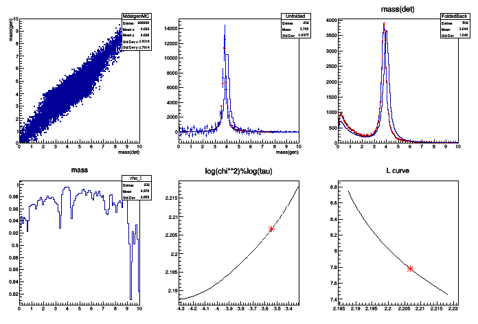
  1. Generate Monte Carlo and Data events The events consist of

    • signal
    • background

    The signal is a resonance. It is generated with a Breit-Wigner, smeared by a Gaussian

  2. Unfold the data. The result is:
    • The background level
    • The shape of the resonance, corrected for detector effects

      The regularisation is done on the curvature, excluding the bins near the peak.

  3. produce some plots

Version 17.0, updated for changed methods in TUnfold

History:

pict1_testUnfold2.C.png
Processing /mnt/vdb/lsf/workspace/root-makedoc-v608/rootspi/rdoc/src/v6-08-00-patches/tutorials/math/testUnfold2.C...
tau=0.000286365
chi**2=160.946+4.9728 / 147
(int) 0
#include <TMath.h>
#include <TCanvas.h>
#include <TRandom3.h>
#include <TFitter.h>
#include <TF1.h>
#include <TStyle.h>
#include <TVector.h>
#include <TGraph.h>
#include "TUnfold.h"
using namespace std;
TRandom *rnd=0;
// generate an event
// output:
// negative mass: background event
// positive mass: signal event
Double_t GenerateEvent(Double_t bgr, // relative fraction of background
Double_t mass, // peak position
Double_t gamma /* peak width*/ )
{
if(rnd->Rndm()>bgr) {
// generate signal event
// with positive mass
do {
do {
t=rnd->Rndm();
} while(t>=1.0);
t=TMath::Tan((t-0.5)*TMath::Pi())*gamma+mass;
} while(t<=0.0);
return t;
} else {
// generate background event
// generate events following a power-law distribution
// f(E) = K * TMath::power((E0+E),N0)
static Double_t const E0=2.4;
static Double_t const N0=2.9;
do {
do {
t=rnd->Rndm();
} while(t>=1.0);
// the mass is returned negative
// In our example a convenient way to indicate it is a background event.
t= -(TMath::Power(1.-t,1./(1.-N0))-1.0)*E0;
} while(t>=0.0);
return t;
}
}
// smear the event to detector level
// input:
// mass on generator level (mTrue>0 !)
// output:
// mass on detector level
Double_t DetectorEvent(Double_t mTrue) {
// smear by double-gaussian
static Double_t frac=0.1;
static Double_t wideBias=0.03;
static Double_t wideSigma=0.5;
static Double_t smallBias=0.0;
static Double_t smallSigma=0.1;
if(rnd->Rndm()>frac) {
return rnd->Gaus(mTrue+smallBias,smallSigma);
} else {
return rnd->Gaus(mTrue+wideBias,wideSigma);
}
}
int testUnfold2()
{
// switch on histogram errors
// random generator
rnd=new TRandom3();
// data and MC luminosity, cross-section
Double_t const luminosityData=100000;
Double_t const luminosityMC=1000000;
Double_t const crossSection=1.0;
Int_t const nDet=250;
Int_t const nGen=100;
Double_t const xminDet=0.0;
Double_t const xmaxDet=10.0;
Double_t const xminGen=0.0;
Double_t const xmaxGen=10.0;
//============================================
// generate MC distribution
//
TH1D *histMgenMC=new TH1D("MgenMC",";mass(gen)",nGen,xminGen,xmaxGen);
TH1D *histMdetMC=new TH1D("MdetMC",";mass(det)",nDet,xminDet,xmaxDet);
TH2D *histMdetGenMC=new TH2D("MdetgenMC",";mass(det);mass(gen)",nDet,xminDet,xmaxDet,
nGen,xminGen,xmaxGen);
Int_t neventMC=rnd->Poisson(luminosityMC*crossSection);
for(Int_t i=0;i<neventMC;i++) {
Double_t mGen=GenerateEvent(0.3, // relative fraction of background
4.0, // peak position in MC
0.2); // peak width in MC
Double_t mDet=DetectorEvent(TMath::Abs(mGen));
// the generated mass is negative for background
// and positive for signal
// so it will be filled in the underflow bin
// this is very convenient for the unfolding:
// the unfolded result will contain the number of background
// events in the underflow bin
// generated MC distribution (for comparison only)
histMgenMC->Fill(mGen,luminosityData/luminosityMC);
// reconstructed MC distribution (for comparison only)
histMdetMC->Fill(mDet,luminosityData/luminosityMC);
// matrix describing how the generator input migrates to the
// reconstructed level. Unfolding input.
// NOTE on underflow/overflow bins:
// (1) the detector level under/overflow bins are used for
// normalisation ("efficiency" correction)
// in our toy example, these bins are populated from tails
// of the initial MC distribution.
// (2) the generator level underflow/overflow bins are
// unfolded. In this example:
// underflow bin: background events reconstructed in the detector
// overflow bin: signal events generated at masses > xmaxDet
// for the unfolded result these bins will be filled
// -> the background normalisation will be contained in the underflow bin
histMdetGenMC->Fill(mDet,mGen,luminosityData/luminosityMC);
}
//============================================
// generate data distribution
//
TH1D *histMgenData=new TH1D("MgenData",";mass(gen)",nGen,xminGen,xmaxGen);
TH1D *histMdetData=new TH1D("MdetData",";mass(det)",nDet,xminDet,xmaxDet);
Int_t neventData=rnd->Poisson(luminosityData*crossSection);
for(Int_t i=0;i<neventData;i++) {
Double_t mGen=GenerateEvent(0.4, // relative fraction of background
3.8, // peak position
0.15); // peak width
Double_t mDet=DetectorEvent(TMath::Abs(mGen));
// generated data mass for comparison plots
// for real data, we do not have this histogram
histMgenData->Fill(mGen);
// reconstructed mass, unfolding input
histMdetData->Fill(mDet);
}
//=========================================================================
// set up the unfolding
TUnfold unfold(histMdetGenMC,TUnfold::kHistMapOutputVert,
// regularisation
//----------------
// the regularisation is done on the curvature (2nd derivative) of
// the output distribution
//
// One has to exclude the bins near the peak of the Breit-Wigner,
// because there the curvature is high
// (and the regularisation eventually could enforce a small
// curvature, thus biasing result)
//
// in real life, the parameters below would have to be optimized,
// depending on the data peak position and width
// Or maybe one finds a different regularisation scheme... this is
// just an example...
Double_t estimatedPeakPosition=3.8;
Int_t nPeek=3;
// calculate bin number correspoinding to estimated peak position
Int_t iPeek=(Int_t)(nGen*(estimatedPeakPosition-xminGen)/(xmaxGen-xminGen)
// offset 1.5
// accounts for start bin 1
// and rounding errors +0.5
+1.5);
// regularize output bins 1..iPeek-nPeek
unfold.RegularizeBins(1,1,iPeek-nPeek,regMode);
// regularize output bins iPeek+nPeek..nGen
unfold.RegularizeBins(iPeek+nPeek,1,nGen-(iPeek+nPeek),regMode);
// unfolding
//-----------
// set input distribution and bias scale (=0)
if(unfold.SetInput(histMdetData,0.0)>=10000) {
std::cout<<"Unfolding result may be wrong\n";
}
// do the unfolding here
Double_t tauMin=0.0;
Double_t tauMax=0.0;
Int_t nScan=30;
Int_t iBest;
TSpline *logTauX,*logTauY;
TGraph *lCurve;
// this method scans the parameter tau and finds the kink in the L curve
// finally, the unfolding is done for the "best" choice of tau
iBest=unfold.ScanLcurve(nScan,tauMin,tauMax,&lCurve,&logTauX,&logTauY);
std::cout<<"tau="<<unfold.GetTau()<<"\n";
std::cout<<"chi**2="<<unfold.GetChi2A()<<"+"<<unfold.GetChi2L()
<<" / "<<unfold.GetNdf()<<"\n";
// save point corresponding to the kink in the L curve as TGraph
Double_t t[1],x[1],y[1];
logTauX->GetKnot(iBest,t[0],x[0]);
logTauY->GetKnot(iBest,t[0],y[0]);
TGraph *bestLcurve=new TGraph(1,x,y);
TGraph *bestLogTauX=new TGraph(1,t,x);
//============================================================
// extract unfolding results into histograms
// set up a bin map, excluding underflow and overflow bins
// the binMap relates the the output of the unfolding to the final
// histogram bins
Int_t *binMap=new Int_t[nGen+2];
for(Int_t i=1;i<=nGen;i++) binMap[i]=i;
binMap[0]=-1;
binMap[nGen+1]=-1;
TH1D *histMunfold=new TH1D("Unfolded",";mass(gen)",nGen,xminGen,xmaxGen);
unfold.GetOutput(histMunfold,binMap);
TH1D *histMdetFold=new TH1D("FoldedBack","mass(det)",nDet,xminDet,xmaxDet);
unfold.GetFoldedOutput(histMdetFold);
// store global correlation coefficients
TH1D *histRhoi=new TH1D("rho_I","mass",nGen,xminGen,xmaxGen);
unfold.GetRhoI(histRhoi,binMap);
delete[] binMap;
binMap=0;
//=====================================================================
// plot some histograms
TCanvas *output = new TCanvas();
// produce some plots
output->Divide(3,2);
// Show the matrix which connects input and output
// There are overflow bins at the bottom, not shown in the plot
// These contain the background shape.
// The overflow bins to the left and right contain
// events which are not reconstructed. These are necessary for proper MC
// normalisation
output->cd(1);
histMdetGenMC->Draw("BOX");
// draw generator-level distribution:
// data (red) [for real data this is not available]
// MC input (black) [with completely wrong peak position and shape]
// unfolded data (blue)
output->cd(2);
histMunfold->SetLineColor(kBlue);
histMunfold->Draw();
histMgenData->SetLineColor(kRed);
histMgenData->Draw("SAME");
histMgenMC->Draw("SAME HIST");
// show detector level distributions
// data (red)
// MC (black)
// unfolded data (blue)
output->cd(3);
histMdetFold->SetLineColor(kBlue);
histMdetFold->Draw();
histMdetData->SetLineColor(kRed);
histMdetData->Draw("SAME");
histMdetMC->Draw("SAME HIST");
// show correlation coefficients
// all bins outside the peak are found to be highly correlated
// But they are compatible with zero anyway
// If the peak shape is fitted,
// these correlations have to be taken into account, see example
output->cd(4);
histRhoi->Draw();
// show rhoi_max(tau) distribution
output->cd(5);
logTauX->Draw();
bestLogTauX->SetMarkerColor(kRed);
bestLogTauX->Draw("*");
output->cd(6);
lCurve->Draw("AL");
bestLcurve->SetMarkerColor(kRed);
bestLcurve->Draw("*");
return 0;
}
Author
Stefan Schmitt, DESY

Definition in file testUnfold2.C.