rs401d_FeldmanCousins.C File Reference

Detailed Description

'Neutrino Oscillation Example from Feldman & Cousins'

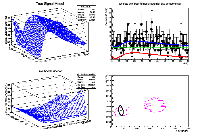
This tutorial shows a more complex example using the FeldmanCousins utility to create a confidence interval for a toy neutrino oscillation experiment. The example attempts to faithfully reproduce the toy example described in Feldman & Cousins' original paper, Phys.Rev.D57:3873-3889,1998.

Processing /mnt/vdb/lsf/workspace/root-makedoc-v608/rootspi/rdoc/src/v6-08-00-patches/tutorials/roostats/rs401d_FeldmanCousins.C...

RooFit v3.60 -- Developed by Wouter Verkerke and David Kirkby 
                Copyright (C) 2000-2013 NIKHEF, University of California & Stanford University
                All rights reserved, please read http://roofit.sourceforge.net/license.txt

RooMsgService::setStreamStatus() ERROR: invalid stream ID 2
generate toy data with nEvents = 692
 **********
 **    1 **SET PRINT           1
 **********
 **********
 **    2 **SET NOGRAD
 **********
 PARAMETER DEFINITIONS:
    NO.   NAME         VALUE      STEP SIZE      LIMITS
     1 deltaMSq     4.00000e+01  1.95000e+01    1.00000e+00  3.00000e+02
     2 sinSq2theta   6.00000e-03  2.00000e-03    0.00000e+00  2.00000e-02
 **********
 **    3 **SET ERR         0.5
 **********
 **********
 **    4 **SET PRINT           1
 **********
 **********
 **    5 **SET STR           1
 **********
 NOW USING STRATEGY  1: TRY TO BALANCE SPEED AGAINST RELIABILITY
 **********
 **    6 **MIGRAD        1000           1
 **********
 FIRST CALL TO USER FUNCTION AT NEW START POINT, WITH IFLAG=4.
 START MIGRAD MINIMIZATION.  STRATEGY  1.  CONVERGENCE WHEN EDM .LT. 1.00e-03
 FCN=-1131.15 FROM MIGRAD    STATUS=INITIATE        8 CALLS           9 TOTAL
                     EDM= unknown      STRATEGY= 1      NO ERROR MATRIX       
  EXT PARAMETER               CURRENT GUESS       STEP         FIRST   
  NO.   NAME      VALUE            ERROR          SIZE      DERIVATIVE 
   1  deltaMSq     4.00000e+01   1.95000e+01   1.99953e-01   1.35503e+01
   2  sinSq2theta   6.00000e-03   2.00000e-03   2.21072e-01  -1.80161e+00
                               ERR DEF= 0.5
 MIGRAD MINIMIZATION HAS CONVERGED.
 MIGRAD WILL VERIFY CONVERGENCE AND ERROR MATRIX.
 COVARIANCE MATRIX CALCULATED SUCCESSFULLY
 FCN=-1131.34 FROM MIGRAD    STATUS=CONVERGED      32 CALLS          33 TOTAL
                     EDM=8.53317e-08    STRATEGY= 1      ERROR MATRIX ACCURATE 
  EXT PARAMETER                                   STEP         FIRST   
  NO.   NAME      VALUE            ERROR          SIZE      DERIVATIVE 
   1  deltaMSq     3.75389e+01   4.12974e+00   9.32732e-04   7.25755e-03
   2  sinSq2theta   6.29097e-03   8.61732e-04   2.04882e-03   6.82825e-04
                               ERR DEF= 0.5
 EXTERNAL ERROR MATRIX.    NDIM=  25    NPAR=  2    ERR DEF=0.5
  1.706e+01 -1.140e-03 
 -1.140e-03  7.447e-07 
 PARAMETER  CORRELATION COEFFICIENTS  
       NO.  GLOBAL      1      2
        1  0.31971   1.000 -0.320
        2  0.31971  -0.320  1.000
 **********
 **    7 **SET ERR         0.5
 **********
 **********
 **    8 **SET PRINT           1
 **********
 **********
 **    9 **HESSE        1000
 **********
 COVARIANCE MATRIX CALCULATED SUCCESSFULLY
 FCN=-1131.34 FROM HESSE     STATUS=OK             10 CALLS          43 TOTAL
                     EDM=8.52816e-08    STRATEGY= 1      ERROR MATRIX ACCURATE 
  EXT PARAMETER                                INTERNAL      INTERNAL  
  NO.   NAME      VALUE            ERROR       STEP SIZE       VALUE   
   1  deltaMSq     3.75389e+01   4.12749e+00   3.73093e-05  -8.56559e-01
   2  sinSq2theta   6.29097e-03   8.61259e-04   4.09765e-04  -3.79981e-01
                               ERR DEF= 0.5
 EXTERNAL ERROR MATRIX.    NDIM=  25    NPAR=  2    ERR DEF=0.5
  1.705e+01 -1.133e-03 
 -1.133e-03  7.439e-07 
 PARAMETER  CORRELATION COEFFICIENTS  
       NO.  GLOBAL      1      2
        1  0.31816   1.000 -0.318
        2  0.31816  -0.318  1.000
[#1] INFO:Minization -- p.d.f. provides expected number of events, including extended term in likelihood.
[#1] INFO:NumericIntegration -- RooRealIntegral::init(PnmuTonePrime_Int[EPrime,LPrime]) using numeric integrator RooAdaptiveIntegratorND to calculate Int(LPrime,EPrime)
[#1] INFO:NumericIntegration -- RooRealIntegral::init(PnmuTone_Int[E,L]) using numeric integrator RooAdaptiveIntegratorND to calculate Int(L,E)
[#1] INFO:NumericIntegration -- RooRealIntegral::init(PnmuTone_Int[L]_Norm[E,L]) using numeric integrator RooIntegrator1D to calculate Int(L)
Metropolis-Hastings progress: ....................................................................................................
[#1] INFO:Eval -- Proposal acceptance rate: 3.3%
[#1] INFO:Eval -- Number of steps in chain: 165
[#1] INFO:NumericIntegration -- RooRealIntegral::init(product_Int[deltaMSq,sinSq2theta]_Norm[deltaMSq,sinSq2theta]) using numeric integrator RooAdaptiveIntegratorND to calculate Int(deltaMSq,sinSq2theta)
[#0] WARNING:NumericIntegration -- RooAdaptiveIntegratorND::dtor(product) WARNING: Number of suppressed warningings about integral evaluations where target precision was not reached is 1
[#1] INFO:NumericIntegration -- RooRealIntegral::init(product_Int[deltaMSq,sinSq2theta]_Norm[deltaMSq,sinSq2theta]) using numeric integrator RooAdaptiveIntegratorND to calculate Int(deltaMSq,sinSq2theta)
[#1] INFO:Eval -- cutoff = 0.166573, conf = 0.904333
[#0] WARNING:NumericIntegration -- RooAdaptiveIntegratorND::dtor(product) WARNING: Number of suppressed warningings about integral evaluations where target precision was not reached is 1
[#0] WARNING:NumericIntegration -- RooAdaptiveIntegratorND::dtor(PnmuTone) WARNING: Number of suppressed warningings about integral evaluations where target precision was not reached is 628
[#0] WARNING:NumericIntegration -- RooAdaptiveIntegratorND::dtor(PnmuTonePrime) WARNING: Number of suppressed warningings about integral evaluations where target precision was not reached is 628
Real time 0:04:13, CP time 253.870
MCMC actual confidence level: 0.904333
[#1] INFO:Minization -- RooProfileLL::evaluate(nll_model_modelData_Profile[deltaMSq,sinSq2theta]) Creating instance of MINUIT
[#1] INFO:Minization -- RooProfileLL::evaluate(nll_model_modelData_Profile[deltaMSq,sinSq2theta]) determining minimum likelihood for current configurations w.r.t all observable
[#1] INFO:Minization -- RooProfileLL::evaluate(nll_model_modelData_Profile[deltaMSq,sinSq2theta]) minimum found at (deltaMSq=37.5376, sinSq2theta=0.00629099)
..[#1] INFO:Minization -- LikelihoodInterval - Finding the contour of deltaMSq ( 0 ) and sinSq2theta ( 1 ) 
Real time 0:05:21, CP time 321.730

#include "RooGlobalFunc.h"
#include "RooStats/ConfInterval.h"
#include "RooStats/FeldmanCousins.h"
#include "RooStats/ProfileLikelihoodCalculator.h"
#include "RooStats/MCMCCalculator.h"
#include "RooStats/UniformProposal.h"
#include "RooStats/LikelihoodIntervalPlot.h"
#include "RooStats/MCMCIntervalPlot.h"
#include "RooStats/MCMCInterval.h"

#include "RooDataSet.h"
#include "RooDataHist.h"
#include "RooRealVar.h"
#include "RooConstVar.h"
#include "RooAddition.h"
#include "RooProduct.h"
#include "RooProdPdf.h"
#include "RooAddPdf.h"

#include "TROOT.h"
#include "RooPolynomial.h"
#include "RooRandom.h"

#include "RooNLLVar.h"
#include "RooProfileLL.h"

#include "RooPlot.h"

#include "TCanvas.h"
#include "TH1F.h"
#include "TH2F.h"
#include "TTree.h"
#include "TMarker.h"
#include "TStopwatch.h"

#include <iostream>

// PDF class created for this macro
#if !defined(__CINT__) || defined(__MAKECINT__)
#include "../tutorials/roostats/NuMuToNuE_Oscillation.h"
#include "../tutorials/roostats/NuMuToNuE_Oscillation.cxx" // so that it can be executed directly
#else
#include "../tutorials/roostats/NuMuToNuE_Oscillation.cxx+" // so that it can be executed directly
#endif

// use this order for safety on library loading
using namespace RooFit;
using namespace RooStats ;


void rs401d_FeldmanCousins(bool doFeldmanCousins=false, bool doMCMC = true)
{

   // to time the macro
   TStopwatch t;
   t.Start();



   // Taken from Feldman & Cousins paper, Phys.Rev.D57:3873-3889,1998.
   // e-Print: physics/9711021 (see page 13.)
   //
   // Quantum mechanics dictates that the probability of such a transformation is given by the formula
   // $P (\nu\mu \rightarrow \nu e ) = sin^2 (2\theta) sin^2 (1.27 \Delta m^2 L /E )$
   // where P is the probability for a $\nu\mu$ to transform into a $\nu e$ , L is the distance in km between
   // the creation of the neutrino from meson decay and its interaction in the detector, E is the
   // neutrino energy in GeV, and $\Delta m^2 = |m^2 - m^2 |$ in $(eV/c^2 )^2$ .
   //
   // To demonstrate how this works in practice, and how it compares to alternative approaches
   // that have been used, we consider a toy model of a typical neutrino oscillation experiment.
   // The toy model is defined by the following parameters: Mesons are assumed to decay to
   // neutrinos uniformly in a region 600 m to 1000 m from the detector. The expected background
   // from conventional $\nu e$ interactions and misidentified $\nu\mu$ interactions is assumed to be 100
   // events in each of 5 energy bins which span the region from 10 to 60 GeV. We assume that
   // the $\nu\mu$ flux is such that if $P (\nu\mu \rightarrow \nu e ) = 0.01$ averaged over any bin, then that bin would
   // have an expected additional contribution of 100 events due to $\nu\mu \rightarrow \nu e$ oscillations.


   // Make signal model model
   RooRealVar E("E","", 15,10,60,"GeV");
   RooRealVar L("L","", .800,.600, 1.0,"km"); // need these units in formula
   RooRealVar deltaMSq("deltaMSq","#Delta m^{2}",40,1,300,"eV/c^{2}");
   RooRealVar sinSq2theta("sinSq2theta","sin^{2}(2#theta)", .006,.0,.02);
   //RooRealVar deltaMSq("deltaMSq","#Delta m^{2}",40,20,70,"eV/c^{2}");
   //  RooRealVar sinSq2theta("sinSq2theta","sin^{2}(2#theta)", .006,.001,.01);
   // PDF for oscillation only describes deltaMSq dependence, sinSq2theta goes into sigNorm
   // 1) The code for this PDF was created by issuing these commands
   //    root [0] RooClassFactory x
   //    root [1] x.makePdf("NuMuToNuE_Oscillation","L,E,deltaMSq","","pow(sin(1.27*deltaMSq*L/E),2)")
   NuMuToNuE_Oscillation PnmuTone("PnmuTone","P(#nu_{#mu} #rightarrow #nu_{e}",L,E,deltaMSq);

   // only E is observable, so create the signal model by integrating out L
   RooAbsPdf* sigModel = PnmuTone.createProjection(L);

   // create  $ \int dE' dL' P(E',L' | \Delta m^2)$.
   // Given RooFit will renormalize the PDF in the range of the observables,
   // the average probability to oscillate in the experiment's acceptance
   // needs to be incorporated into the extended term in the likelihood.
   // Do this by creating a RooAbsReal representing the integral and divide by
   // the area in the E-L plane.
   // The integral should be over "primed" observables, so we need
   // an independent copy of PnmuTone not to interfere with the original.

   // Independent copy for Integral
   RooRealVar EPrime("EPrime","", 15,10,60,"GeV");
   RooRealVar LPrime("LPrime","", .800,.600, 1.0,"km"); // need these units in formula
   NuMuToNuE_Oscillation PnmuTonePrime("PnmuTonePrime","P(#nu_{#mu} #rightarrow #nu_{e}",
                                       LPrime,EPrime,deltaMSq);
   RooAbsReal* intProbToOscInExp = PnmuTonePrime.createIntegral(RooArgSet(EPrime,LPrime));

   // Getting the flux is a bit tricky.  It is more clear to include a cross section term that is not
   // explicitly referred to in the text, eg.
   // number events in bin = flux * cross-section for nu_e interaction in E bin * average prob nu_mu osc. to nu_e in bin
   // let maxEventsInBin = flux * cross-section for nu_e interaction in E bin
   // maxEventsInBin * 1% chance per bin =  100 events / bin
   // therefore maxEventsInBin = 10,000.
   // for 5 bins, this means maxEventsTot = 50,000
   RooConstVar maxEventsTot("maxEventsTot","maximum number of sinal events",50000);
   RooConstVar inverseArea("inverseArea","1/(#Delta E #Delta L)",
                           1./(EPrime.getMax()-EPrime.getMin())/(LPrime.getMax()-LPrime.getMin()));

   // $sigNorm = maxEventsTot \cdot \int dE dL \frac{P_{oscillate\ in\ experiment}}{Area} \cdot {sin}^2(2\theta)$
   RooProduct sigNorm("sigNorm", "", RooArgSet(maxEventsTot, *intProbToOscInExp, inverseArea, sinSq2theta));
   // bkg = 5 bins * 100 events / bin
   RooConstVar bkgNorm("bkgNorm","normalization for background",500);

   // flat background (0th order polynomial, so no arguments for coefficients)
   RooPolynomial bkgEShape("bkgEShape","flat bkg shape", E);

   // total model
   RooAddPdf model("model","",RooArgList(*sigModel,bkgEShape),
                     RooArgList(sigNorm,bkgNorm));

   // for debugging, check model tree
   //  model.printCompactTree();
   //  model.graphVizTree("model.dot");


   // turn off some messages
   RooMsgService::instance().setStreamStatus(0,kFALSE);
   RooMsgService::instance().setStreamStatus(1,kFALSE);
   RooMsgService::instance().setStreamStatus(2,kFALSE);


   // --------------------------------------
   // n events in data to data, simply sum of sig+bkg
   Int_t nEventsData = bkgNorm.getVal()+sigNorm.getVal();
   cout << "generate toy data with nEvents = " << nEventsData << endl;
   // adjust random seed to get a toy dataset similar to one in paper.
   // Found by trial and error (3 trials, so not very "fine tuned")
   RooRandom::randomGenerator()->SetSeed(3);
   // create a toy dataset
   RooDataSet* data = model.generate(RooArgSet(E), nEventsData);

   // --------------------------------------
   // make some plots
   TCanvas* dataCanvas = new TCanvas("dataCanvas");
   dataCanvas->Divide(2,2);

   // plot the PDF
   dataCanvas->cd(1);
   TH1* hh = PnmuTone.createHistogram("hh",E,Binning(40),YVar(L,Binning(40)),Scaling(kFALSE)) ;
   hh->SetLineColor(kBlue) ;
   hh->SetTitle("True Signal Model");
   hh->Draw("surf");

   // plot the data with the best fit
   dataCanvas->cd(2);
   RooPlot* Eframe = E.frame();
   data->plotOn(Eframe);
   model.fitTo(*data, Extended());
   model.plotOn(Eframe);
   model.plotOn(Eframe,Components(*sigModel),LineColor(kRed));
   model.plotOn(Eframe,Components(bkgEShape),LineColor(kGreen));
   model.plotOn(Eframe);
   Eframe->SetTitle("toy data with best fit model (and sig+bkg components)");
   Eframe->Draw();

   // plot the likelihood function
   dataCanvas->cd(3);
   RooNLLVar nll("nll", "nll", model, *data, Extended());
   RooProfileLL pll("pll", "", nll, RooArgSet(deltaMSq, sinSq2theta));
   //  TH1* hhh = nll.createHistogram("hhh",sinSq2theta,Binning(40),YVar(deltaMSq,Binning(40))) ;
   TH1* hhh = pll.createHistogram("hhh",sinSq2theta,Binning(40),YVar(deltaMSq,Binning(40)),Scaling(kFALSE)) ;
   hhh->SetLineColor(kBlue) ;
   hhh->SetTitle("Likelihood Function");
   hhh->Draw("surf");

   dataCanvas->Update();



   // --------------------------------------------------------------
   // show use of Feldman-Cousins utility in RooStats
   // set the distribution creator, which encodes the test statistic
   RooArgSet parameters(deltaMSq, sinSq2theta);
   RooWorkspace* w = new RooWorkspace();

   ModelConfig modelConfig;
   modelConfig.SetWorkspace(*w);
   modelConfig.SetPdf(model);
   modelConfig.SetParametersOfInterest(parameters);

   RooStats::FeldmanCousins fc(*data, modelConfig);
   fc.SetTestSize(.1); // set size of test
   fc.UseAdaptiveSampling(true);
   fc.SetNBins(10); // number of points to test per parameter

   // use the Feldman-Cousins tool
   ConfInterval* interval = 0;
   if(doFeldmanCousins)
      interval = fc.GetInterval();


   // ---------------------------------------------------------
   // show use of ProfileLikeihoodCalculator utility in RooStats
   RooStats::ProfileLikelihoodCalculator plc(*data, modelConfig);
   plc.SetTestSize(.1);

   ConfInterval* plcInterval = plc.GetInterval();

   // --------------------------------------------
   // show use of MCMCCalculator utility in RooStats
   MCMCInterval* mcInt = NULL;

   if (doMCMC) {
         // turn some messages back on
         RooMsgService::instance().setStreamStatus(0,kTRUE);
         RooMsgService::instance().setStreamStatus(1,kTRUE);

         TStopwatch mcmcWatch;
         mcmcWatch.Start();

         RooArgList axisList(deltaMSq, sinSq2theta);
         MCMCCalculator mc(*data, modelConfig);
         mc.SetNumIters(5000);
         mc.SetNumBurnInSteps(100);
         mc.SetUseKeys(true);
         mc.SetTestSize(.1);
         mc.SetAxes(axisList); // set which is x and y axis in posterior histogram
         //mc.SetNumBins(50);
         mcInt = (MCMCInterval*)mc.GetInterval();

         mcmcWatch.Stop();
         mcmcWatch.Print();
   }
   // -------------------------------
   // make plot of resulting interval

   dataCanvas->cd(4);

   // first plot a small dot for every point tested
   if (doFeldmanCousins) {
      RooDataHist* parameterScan = (RooDataHist*) fc.GetPointsToScan();
      TH2F* hist = (TH2F*) parameterScan->createHistogram("sinSq2theta:deltaMSq",30,30);
      //  hist->Draw();
      TH2F* forContour = (TH2F*)hist->Clone();

      // now loop through the points and put a marker if it's in the interval
      RooArgSet* tmpPoint;
      // loop over points to test
      for(Int_t i=0; i<parameterScan->numEntries(); ++i){
         // get a parameter point from the list of points to test.
         tmpPoint = (RooArgSet*) parameterScan->get(i)->clone("temp");

         if (interval){
            if (interval->IsInInterval( *tmpPoint ) ) {
               forContour->SetBinContent( hist->FindBin(tmpPoint->getRealValue("sinSq2theta"),
                        tmpPoint->getRealValue("deltaMSq")), 1);
            }else{
               forContour->SetBinContent( hist->FindBin(tmpPoint->getRealValue("sinSq2theta"),
                        tmpPoint->getRealValue("deltaMSq")), 0);
            }
         }


         delete tmpPoint;
      }

      if (interval){
         Double_t level=0.5;
         forContour->SetContour(1,&level);
         forContour->SetLineWidth(2);
         forContour->SetLineColor(kRed);
         forContour->Draw("cont2,same");
      }
   }

   MCMCIntervalPlot* mcPlot = NULL;
   if (mcInt) {
      cout << "MCMC actual confidence level: "
         << mcInt->GetActualConfidenceLevel() << endl;
      mcPlot = new MCMCIntervalPlot(*mcInt);
      mcPlot->SetLineColor(kMagenta);
      mcPlot->Draw();
   }
   dataCanvas->Update();

   LikelihoodIntervalPlot plotInt((LikelihoodInterval*)plcInterval);
   plotInt.SetTitle("90% Confidence Intervals");
   if (mcInt)
      plotInt.Draw("same");
   else
      plotInt.Draw();
   dataCanvas->Update();

   /// print timing info
   t.Stop();
   t.Print();


}

Author

Kyle Cranmer

Definition in file rs401d_FeldmanCousins.C.