Processing /mnt/vdb/lsf/workspace/root-makedoc-v608/rootspi/rdoc/src/v6-08-00-patches/tutorials/roofit/rf610_visualerror.C...
�[1mRooFit v3.60 -- Developed by Wouter Verkerke and David Kirkby�[0m
Copyright (C) 2000-2013 NIKHEF, University of California & Stanford University
All rights reserved, please read http://roofit.sourceforge.net/license.txt
[#1] INFO:Minization -- RooMinimizer::optimizeConst: activating const optimization
[#1] INFO:Minization -- The following expressions will be evaluated in cache-and-track mode: (sig,bkg)
**********
** 1 **SET PRINT 1
**********
**********
** 2 **SET NOGRAD
**********
PARAMETER DEFINITIONS:
NO. NAME VALUE STEP SIZE LIMITS
1 fsig 3.30000e-01 1.00000e-01 0.00000e+00 1.00000e+00
2 m 0.00000e+00 2.00000e+00 -1.00000e+01 1.00000e+01
3 m2 -1.00000e+00 2.00000e+00 -1.00000e+01 1.00000e+01
4 s 2.00000e+00 5.00000e-01 1.00000e+00 5.00000e+01
5 s2 6.00000e+00 2.50000e+00 1.00000e+00 5.00000e+01
**********
** 3 **SET ERR 0.5
**********
**********
** 4 **SET PRINT 1
**********
**********
** 5 **SET STR 1
**********
NOW USING STRATEGY 1: TRY TO BALANCE SPEED AGAINST RELIABILITY
**********
** 6 **MIGRAD 2500 1
**********
FIRST CALL TO USER FUNCTION AT NEW START POINT, WITH IFLAG=4.
START MIGRAD MINIMIZATION. STRATEGY 1. CONVERGENCE WHEN EDM .LT. 1.00e-03
FCN=2770.05 FROM MIGRAD STATUS=INITIATE 20 CALLS 21 TOTAL
EDM= unknown STRATEGY= 1 NO ERROR MATRIX
EXT PARAMETER CURRENT GUESS STEP FIRST
NO. NAME VALUE ERROR SIZE DERIVATIVE
1 fsig 3.30000e-01 1.00000e-01 2.14988e-01 -9.80006e+00
2 m 0.00000e+00 2.00000e+00 2.01358e-01 -3.95919e+01
3 m2 -1.00000e+00 2.00000e+00 2.02430e-01 3.98515e+01
4 s 2.00000e+00 5.00000e-01 7.46809e-02 2.95415e+01
5 s2 6.00000e+00 2.50000e+00 1.74125e-01 4.56667e+01
ERR DEF= 0.5
MIGRAD MINIMIZATION HAS CONVERGED.
MIGRAD WILL VERIFY CONVERGENCE AND ERROR MATRIX.
COVARIANCE MATRIX CALCULATED SUCCESSFULLY
FCN=2767.65 FROM MIGRAD STATUS=CONVERGED 125 CALLS 126 TOTAL
EDM=1.56678e-05 STRATEGY= 1 ERROR MATRIX ACCURATE
EXT PARAMETER STEP FIRST
NO. NAME VALUE ERROR SIZE DERIVATIVE
1 fsig 2.98883e-01 6.74303e-02 2.39863e-03 7.00359e-03
2 m 3.08816e-01 2.09098e-01 6.83546e-04 -2.93512e-02
3 m2 -1.31219e+00 3.64277e-01 9.46152e-04 8.97852e-02
4 s 1.78229e+00 2.51997e-01 9.25951e-04 -2.49363e-02
5 s2 5.51197e+00 4.85498e-01 6.94615e-04 1.27501e-01
ERR DEF= 0.5
EXTERNAL ERROR MATRIX. NDIM= 25 NPAR= 5 ERR DEF=0.5
4.580e-03 -3.800e-03 -1.557e-02 1.331e-02 2.642e-02
-3.800e-03 4.373e-02 -3.141e-03 -1.195e-02 -2.959e-02
-1.557e-02 -3.141e-03 1.328e-01 -4.509e-02 -1.100e-01
1.331e-02 -1.195e-02 -4.509e-02 6.354e-02 7.253e-02
2.642e-02 -2.959e-02 -1.100e-01 7.253e-02 2.358e-01
PARAMETER CORRELATION COEFFICIENTS
NO. GLOBAL 1 2 3 4 5
1 0.89430 1.000 -0.269 -0.632 0.780 0.804
2 0.43384 -0.269 1.000 -0.041 -0.227 -0.291
3 0.70478 -0.632 -0.041 1.000 -0.491 -0.621
4 0.78303 0.780 -0.227 -0.491 1.000 0.593
5 0.82883 0.804 -0.291 -0.621 0.593 1.000
**********
** 7 **SET ERR 0.5
**********
**********
** 8 **SET PRINT 1
**********
**********
** 9 **HESSE 2500
**********
COVARIANCE MATRIX CALCULATED SUCCESSFULLY
FCN=2767.65 FROM HESSE STATUS=OK 31 CALLS 157 TOTAL
EDM=1.56685e-05 STRATEGY= 1 ERROR MATRIX ACCURATE
EXT PARAMETER INTERNAL INTERNAL
NO. NAME VALUE ERROR STEP SIZE VALUE
1 fsig 2.98883e-01 6.78952e-02 4.79727e-04 -4.13956e-01
2 m 3.08816e-01 2.09026e-01 1.36709e-04 3.08865e-02
3 m2 -1.31219e+00 3.67042e-01 1.89230e-04 -1.31599e-01
4 s 1.78229e+00 2.53102e-01 1.85190e-04 -1.31741e+00
5 s2 5.51197e+00 4.89300e-01 1.38923e-04 -9.54177e-01
ERR DEF= 0.5
EXTERNAL ERROR MATRIX. NDIM= 25 NPAR= 5 ERR DEF=0.5
4.644e-03 -3.811e-03 -1.596e-02 1.350e-02 2.692e-02
-3.811e-03 4.370e-02 -2.970e-03 -1.206e-02 -2.967e-02
-1.596e-02 -2.970e-03 1.348e-01 -4.619e-02 -1.129e-01
1.350e-02 -1.206e-02 -4.619e-02 6.410e-02 7.402e-02
2.692e-02 -2.967e-02 -1.129e-01 7.402e-02 2.395e-01
PARAMETER CORRELATION COEFFICIENTS
NO. GLOBAL 1 2 3 4 5
1 0.89584 1.000 -0.268 -0.638 0.782 0.807
2 0.43319 -0.268 1.000 -0.039 -0.228 -0.290
3 0.71012 -0.638 -0.039 1.000 -0.497 -0.628
4 0.78518 0.782 -0.228 -0.497 1.000 0.597
5 0.83175 0.807 -0.290 -0.628 0.597 1.000
[#1] INFO:Minization -- RooMinimizer::optimizeConst: deactivating const optimization
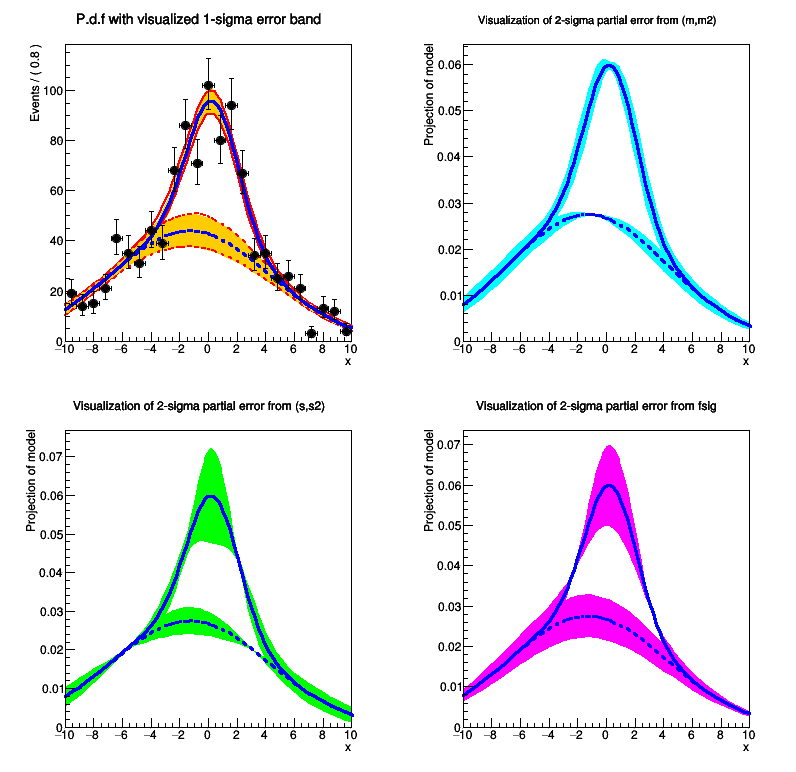
[#1] INFO:Plotting -- RooAbsReal::plotOn(model) INFO: visualizing 1-sigma uncertainties in parameters (m,s,fsig,m2,s2) from fit result fitresult_model_genData using 315 samplings.
[#1] INFO:Plotting -- RooAbsPdf::plotOn(model) directly selected PDF components: (bkg)
[#1] INFO:Plotting -- RooAbsPdf::plotOn(model) indirectly selected PDF components: ()
[#1] INFO:Plotting -- RooAbsPdf::plotOn(model) directly selected PDF components: (bkg)
[#1] INFO:Plotting -- RooAbsPdf::plotOn(model) indirectly selected PDF components: ()
[#1] INFO:Plotting -- RooAbsPdf::plotOn(model) directly selected PDF components: (bkg)
[#1] INFO:Plotting -- RooAbsPdf::plotOn(model) indirectly selected PDF components: ()
[#1] INFO:Plotting -- RooAbsPdf::plotOn(model) directly selected PDF components: (bkg)
[#1] INFO:Plotting -- RooAbsPdf::plotOn(model) indirectly selected PDF components: ()
[#1] INFO:Plotting -- RooAbsPdf::plotOn(model) directly selected PDF components: (bkg)
[#1] INFO:Plotting -- RooAbsPdf::plotOn(model) indirectly selected PDF components: ()
[#1] INFO:Plotting -- RooAbsPdf::plotOn(model) directly selected PDF components: (bkg)
[#1] INFO:Plotting -- RooAbsPdf::plotOn(model) indirectly selected PDF components: ()
[#1] INFO:Plotting -- RooAbsPdf::plotOn(model) directly selected PDF components: (bkg)
[#1] INFO:Plotting -- RooAbsPdf::plotOn(model) indirectly selected PDF components: ()


 ROOT 6.07/09 - Reference Guide Generated on Wed Oct 19 2016 02:19:47 using Doxygen 1.8.12.

