mlpHiggs.C File Reference

Detailed Description

Example of a Multi Layer Perceptron For a LEP search for invisible Higgs boson, a neural network was used to separate the signal from the background passing some selection cuts.

Here is a simplified version of this network, taking into account only WW events.

Processing /mnt/vdb/lsf/workspace/root-makedoc-v608/rootspi/rdoc/src/v6-08-00-patches/tutorials/mlp/mlpHiggs.C...
accessing mlpHiggs.root file from http://root.cern.ch/files
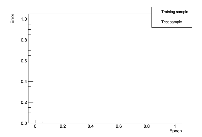
Training the Neural Network
Epoch: 0 learn=0.126964 test=0.126101
Epoch: 10 learn=0.099816 test=0.0944112
Epoch: 20 learn=0.0967496 test=0.0914356
Epoch: 30 learn=0.0957444 test=0.0902211
Epoch: 40 learn=0.0929555 test=0.089151
Epoch: 50 learn=0.0922609 test=0.0886525
Epoch: 60 learn=0.0916939 test=0.0882441
Epoch: 70 learn=0.0910837 test=0.0879216
Epoch: 80 learn=0.0907021 test=0.0880823
Epoch: 90 learn=0.0901749 test=0.086813
Epoch: 99 learn=0.0901028 test=0.0863809
Training done.
test.py created.
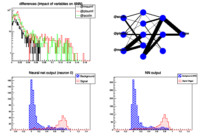
Network with structure: @msumf,@ptsumf,@acolin:5:3:type
inputs with low values in the differences plot may not be needed
@msumf -> 0.016667 +/- 0.0132143
@ptsumf -> 0.0267861 +/- 0.0378194
@acolin -> 0.025739 +/- 0.0295963

void mlpHiggs(Int_t ntrain=100) {
   const char *fname = "mlpHiggs.root";
   TFile *input = 0;
   if (!gSystem->AccessPathName(fname)) {
      input = TFile::Open(fname);
   } else {
      printf("accessing %s file from http://root.cern.ch/files\n",fname);
      input = TFile::Open(Form("http://root.cern.ch/files/%s",fname));
   }
   if (!input) return;

   TTree *sig_filtered = (TTree *) input->Get("sig_filtered");
   TTree *bg_filtered = (TTree *) input->Get("bg_filtered");
   TTree *simu = new TTree("MonteCarlo", "Filtered Monte Carlo Events");
   Float_t ptsumf, qelep, nch, msumf, minvis, acopl, acolin;
   Int_t type;
   sig_filtered->SetBranchAddress("ptsumf", &ptsumf);
   sig_filtered->SetBranchAddress("qelep",  &qelep);
   sig_filtered->SetBranchAddress("nch",    &nch);
   sig_filtered->SetBranchAddress("msumf",  &msumf);
   sig_filtered->SetBranchAddress("minvis", &minvis);
   sig_filtered->SetBranchAddress("acopl",  &acopl);
   sig_filtered->SetBranchAddress("acolin", &acolin);
   bg_filtered->SetBranchAddress("ptsumf", &ptsumf);
   bg_filtered->SetBranchAddress("qelep",  &qelep);
   bg_filtered->SetBranchAddress("nch",    &nch);
   bg_filtered->SetBranchAddress("msumf",  &msumf);
   bg_filtered->SetBranchAddress("minvis", &minvis);
   bg_filtered->SetBranchAddress("acopl",  &acopl);
   bg_filtered->SetBranchAddress("acolin", &acolin);
   simu->Branch("ptsumf", &ptsumf, "ptsumf/F");
   simu->Branch("qelep",  &qelep,  "qelep/F");
   simu->Branch("nch",    &nch,    "nch/F");
   simu->Branch("msumf",  &msumf,  "msumf/F");
   simu->Branch("minvis", &minvis, "minvis/F");
   simu->Branch("acopl",  &acopl,  "acopl/F");
   simu->Branch("acolin", &acolin, "acolin/F");
   simu->Branch("type",   &type,   "type/I");
   type = 1;
   Int_t i;
   for (i = 0; i < sig_filtered->GetEntries(); i++) {
      sig_filtered->GetEntry(i);
      simu->Fill();
   }
   type = 0;
   for (i = 0; i < bg_filtered->GetEntries(); i++) {
      bg_filtered->GetEntry(i);
      simu->Fill();
   }
   // Build and train the NN ptsumf is used as a weight since we are primarily
   // interested  by high pt events.
   // The datasets used here are the same as the default ones.
   TMultiLayerPerceptron *mlp =
      new TMultiLayerPerceptron("@msumf,@ptsumf,@acolin:5:3:type",
                                "ptsumf",simu,"Entry$%2","(Entry$+1)%2");
   mlp->Train(ntrain, "text,graph,update=10");
   mlp->Export("test","python");
   // Use TMLPAnalyzer to see what it looks for
   TCanvas* mlpa_canvas = new TCanvas("mlpa_canvas","Network analysis");
   mlpa_canvas->Divide(2,2);
   TMLPAnalyzer ana(mlp);
   // Initialisation
   ana.GatherInformations();
   // output to the console
   ana.CheckNetwork();
   mlpa_canvas->cd(1);
   // shows how each variable influences the network
   ana.DrawDInputs();
   mlpa_canvas->cd(2);
   // shows the network structure
   mlp->Draw();
   mlpa_canvas->cd(3);
   // draws the resulting network
   ana.DrawNetwork(0,"type==1","type==0");
   mlpa_canvas->cd(4);
   // Use the NN to plot the results for each sample
   // This will give approx. the same result as DrawNetwork.
   // All entries are used, while DrawNetwork focuses on
   // the test sample. Also the xaxis range is manually set.
   TH1F *bg = new TH1F("bgh", "NN output", 50, -.5, 1.5);
   TH1F *sig = new TH1F("sigh", "NN output", 50, -.5, 1.5);
   bg->SetDirectory(0);
   sig->SetDirectory(0);
   Double_t params[3];
   for (i = 0; i < bg_filtered->GetEntries(); i++) {
      bg_filtered->GetEntry(i);
      params[0] = msumf;
      params[1] = ptsumf;
      params[2] = acolin;
      bg->Fill(mlp->Evaluate(0, params));
   }
   for (i = 0; i < sig_filtered->GetEntries(); i++) {
      sig_filtered->GetEntry(i);
      params[0] = msumf;
      params[1] = ptsumf;
      params[2] = acolin;
      sig->Fill(mlp->Evaluate(0,params));
   }
   bg->SetLineColor(kBlue);
   bg->SetFillStyle(3008);   bg->SetFillColor(kBlue);
   sig->SetLineColor(kRed);
   sig->SetFillStyle(3003); sig->SetFillColor(kRed);
   bg->SetStats(0);
   sig->SetStats(0);
   bg->Draw();
   sig->Draw("same");
   TLegend *legend = new TLegend(.75, .80, .95, .95);
   legend->AddEntry(bg, "Background (WW)");
   legend->AddEntry(sig, "Signal (Higgs)");
   legend->Draw();
   mlpa_canvas->cd(0);
   delete input;
}

Author

Christophe Delaere

Definition in file mlpHiggs.C.