portfolio.C: This macro shows in detail the use of the quadratic programming package quadp .
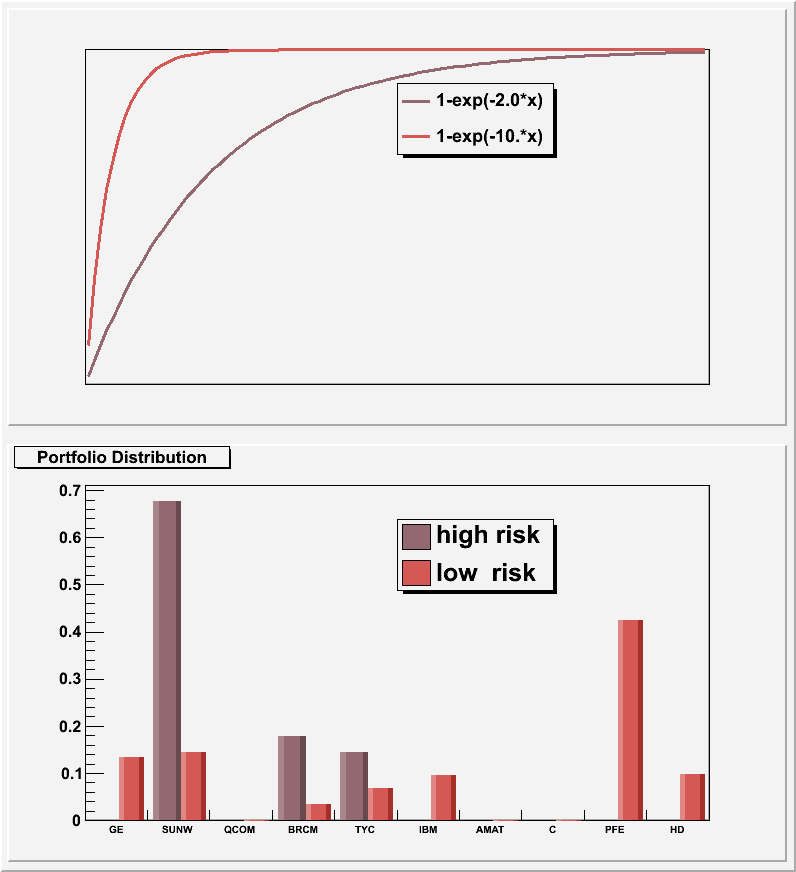
#include "Riostream.h" #include "TCanvas.h" #include "TFile.h" #include "TMath.h" #include "TTree.h" #include "TArrayF.h" #include "TH1.h" #include "TF1.h" #include "TLegend.h" #include "TSystem.h" #include "TMatrixD.h" #include "TMatrixDSym.h" #include "TVectorD.h" #include "TQpProbDens.h" #include "TGondzioSolver.h" //+ This macro shows in detail the use of the quadratic programming package quadp . // Running this macro : // .x portfolio.C+ // or gSystem->Load("libQuadp"); .L portFolio.C+; portfolio() // // Let's first review what we exactly mean by "quadratic programming" : // // We want to minimize the following objective function : // // c^T x + ( 1/2 ) x^T Q x wrt. the vector x // // c is a vector and Q a symmetric positive definite matrix // // You might wonder what is so special about this objective which is quadratic in // the unknowns, that can not be done by Minuit/Fumili . Well, we have in addition // the following boundary conditions on x: // // A x = b // clo <= C x <= cup // xlo <= x <= xup , where A and C are arbitray matrices and the rest are vectors // // Not all these constraints have to be defined . Our example will only use xlo, A and b // Still, this could be handled by a general non-linear minimizer like Minuit by introducing // so-called "slack" variables . However, quadp is tailored to objective functions not more // complex than being quadratic . This allows usage of solving techniques which are even // stable for problems involving for instance 500 variables, 100 inequality conditions // and 50 equality conditions . // // Enough said about quadratic programming, let's return to our example . // Suppose, after a long day of doing physics, you have a look at your investments and // realize that an early retirement is not possible, given the returns of your stocks . // So what now ? ROOT to the rescue ...... // // In 1990 Harry Markowitz was awarded the Noble prize for economics : " his work provided new tools // for weighing the risks and rewards of different investments and for valuing corporate stocks and bonds" . // In plain English, he developed the tools to balance greed and fear, we want the maximum return // with the minimum amount of risk. Our stock portfolio should be at the "Efficient Frontier", // see http://www.riskglossary.com/articles/efficient_frontier.htm . // To quantify better the risk we are willing to take, we define a utility function U(x) . It describes // as a function of our total assets x, our "satisfaction" . A common choice is 1-exp(-k*x) (the reason for // the exponent will be clear later) . The parameter k is the risk-aversion factor . For small values of k // the satisfaction is small for small values of x; by increasing x the satisfaction can still be increased // significantly . For large values of k, U(x) increases rapidly to 1, there is no increase in satisfaction // for additional dollars earned . // // In summary : small k ==> risk-loving investor // large k ==> risk-averse investor // // Suppose we have for nrStocks the historical daily returns r = closing_price(n) - closing_price(n-1) . // Define a vector x of length of nrStocks, which contains the fraction of our money invested in // each stock . We can calculate the average daily return z of our portfolio and its variance using // the portfolio covariance Covar : // // z = r^T x and var = x^T Covar x // // Assuming that the daily returns have a Normal distribution, N(x), so will z with mean r^T x // and variance x^T Covar x // // The expected value of the utility function is : E(u(x)) = Int (1-exp(-k*x) N(x) dx // = 1-exp(-k (r^T x - 0.5 k x^T Covar x) ) // // Its value is maximized by maximizing r^T x -0.5 k x^T Covar x // under the condition sum (x_i) = 1, meaning we want all our money invested and // x_i >= 0 , we can not "short" a stock // // For 10 stocks we got the historical daily data for Sep-2000 to Jun-2004: // // GE : General Electric Co // SUNW : Sun Microsystems Inc // QCOM : Qualcomm Inc // BRCM : Broadcom Corp // TYC : Tyco International Ltd // IBM : International Business Machines Corp // AMAT : Applied Materials Inc // C : Citigroup Inc // PFE : Pfizer Inc // HD : Home Depot Inc // // We calculate the optimal portfolio for 2.0 and 10.0 . // // Food for thought : // - We assumed that the stock returns have a Normal distribution . Check this assumption by // histogramming the stock returns ! // - We used for the expected return in the objective function, the flat average over a time // period . Investment firms will put significant resources in improving the return predicton . // - If you want to trade significant number of shares, several other considerations have // to be taken into account : // + If you are going to buy, you will drive the price up (so-called "slippage") . // This can be taken into account by adding terms to the objective // (Google for "slippage optimization") // + FTC regulations might have to be added to the inequality constraints // - Investment firms do not want to be exposed to the "market" as defined by a broad // index like the S&P and "hedge" this exposure away . A perfect hedge this can be added // as an equality constrain, otherwise add an inequality constrain . // //Author: Eddy Offermann const Int_t nrStocks = 10; static const Char_t *stocks[] = {"GE","SUNW","QCOM","BRCM","TYC","IBM","AMAT","C","PFE","HD"}; class TStockDaily { public: Int_t fDate; Int_t fOpen; // 100*open_price Int_t fHigh; // 100*high_price Int_t fLow; // 100*low_price Int_t fClose; // 100*close_price Int_t fVol; Int_t fCloseAdj; // 100*close_price adjusted for splits and dividend TStockDaily() { fDate = fVol = fOpen = fHigh = fLow = fClose = fCloseAdj = 0; } virtual ~TStockDaily() {} ClassDef(TStockDaily,1) }; //--------------------------------------------------------------------------- Double_t RiskProfile(Double_t *x, Double_t *par) { Double_t riskFactor = par[0]; return 1-TMath::Exp(-riskFactor*x[0]); } //--------------------------------------------------------------------------- TArrayF &StockReturn(TFile *f,const TString &name,Int_t sDay,Int_t eDay) { TTree *tDaily = (TTree*)f->Get(name); TStockDaily *data = 0; tDaily->SetBranchAddress("daily",&data); TBranch *b_closeAdj = tDaily->GetBranch("fCloseAdj"); TBranch *b_date = tDaily->GetBranch("fDate"); //read only the "adjusted close" branch for all entries const Int_t nrEntries = (Int_t)tDaily->GetEntries(); TArrayF closeAdj(nrEntries); for (Int_t i = 0; i < nrEntries; i++) { b_date->GetEntry(i); b_closeAdj->GetEntry(i); if (data->fDate >= sDay && data->fDate <= eDay) #ifdef __CINT__ closeAdj.AddAt(data->fCloseAdj/100. , i ); #else closeAdj[i] = data->fCloseAdj/100.; #endif } TArrayF *r = new TArrayF(nrEntries-1); for (Int_t i = 1; i < nrEntries; i++) // (*r)[i-1] = closeAdj[i]-closeAdj[i-1]; #ifdef __CINT__ r->AddAt(closeAdj[i]/closeAdj[i-1],1); #else (*r)[i-1] = closeAdj[i]/closeAdj[i-1]; #endif return *r; } #ifndef __MAKECINT__ //--------------------------------------------------------------------------- TVectorD OptimalInvest(Double_t riskFactor,TVectorD r,TMatrixDSym Covar) { // what the quadratic programming package will do: // // minimize c^T x + ( 1/2 ) x^T Q x // subject to A x = b // clo <= C x <= cup // xlo <= x <= xup // what we want : // // maximize c^T x - k ( 1/2 ) x^T Q x // subject to sum_x x_i = 1 // 0 <= x_i // We have nrStocks weights to determine, // 1 equality- and 0 inequality- equations (the simple square boundary // condition (xlo <= x <= xup) does not count) const Int_t nrVar = nrStocks; const Int_t nrEqual = 1; const Int_t nrInEqual = 0; // flip the sign of the objective function because we want to maximize TVectorD c = -1.*r; TMatrixDSym Q = riskFactor*Covar; // equality equation TMatrixD A(nrEqual,nrVar); A = 1; TVectorD b(nrEqual); b = 1; // inequality equation // // - although not applicable in the current situatio since nrInEqual = 0, one // has to specify not only clo and cup but also an index vector iclo and icup, // whose values are either 0 or 1 . If iclo[j] = 1, the lower boundary condition // is active on x[j], etc. ... TMatrixD C (nrInEqual,nrVar); TVectorD clo (nrInEqual); TVectorD cup (nrInEqual); TVectorD iclo(nrInEqual); TVectorD icup(nrInEqual); // simple square boundary condition : 0 <= x_i, so only xlo is relevant . // Like for clo and cup above, we have to define an index vector ixlo and ixup . // Since each variable has the lower boundary, we can set the whole vector // ixlo = 1 TVectorD xlo (nrVar); xlo = 0; TVectorD xup (nrVar); xup = 0; TVectorD ixlo(nrVar); ixlo = 1; TVectorD ixup(nrVar); ixup = 0; // setup the quadratic programming problem . Since a small number of variables are // involved and "Q" has everywhere entries, we chose the dense version "TQpProbDens" . // In case of a sparse formulation, simply replace all "Dens" by "Sparse" below and // use TMatrixDSparse instead of TMatrixDSym and TMatrixD TQpProbDens *qp = new TQpProbDens(nrVar,nrEqual,nrInEqual); // stuff all the matrices/vectors defined above in the proper places TQpDataDens *prob = (TQpDataDens *)qp->MakeData(c,Q,xlo,ixlo,xup,ixup,A,b,C,clo,iclo,cup,icup); // setup the nrStock variables, vars->fX will contain the final solution TQpVar *vars = qp->MakeVariables(prob); TQpResidual *resid = qp->MakeResiduals(prob); // Now we have to choose the method of solving, either TGondzioSolver or TMehrotraSolver // The Gondzio method is more sophisticated and therefore numerically more involved // If one want the Mehrotra method, simply replace "Gondzio" by "Mehrotra" . TGondzioSolver *s = new TGondzioSolver(qp,prob); const Int_t status = s->Solve(prob,vars,resid); const TVectorD weight = vars->fX; delete qp; delete prob; delete vars; delete resid; delete s; if (status != 0) { cout << "Could not solve this problem." <<endl; return TVectorD(nrStocks); } return weight; } #endif //--------------------------------------------------------------------------- void portfolio() { const Int_t sDay = 20000809; const Int_t eDay = 20040602; const char *fname = "stock.root"; TFile *f = 0; if (!gSystem->AccessPathName(fname)) { f = TFile::Open(fname); } else { printf("accessing %s file from http://root.cern.ch/files\n",fname); f = TFile::Open(Form("http://root.cern.ch/files/%s",fname)); } if (!f) return; TArrayF *data = new TArrayF[nrStocks]; for (Int_t i = 0; i < nrStocks; i++) { const TString symbol = stocks[i]; data[i] = StockReturn(f,symbol,sDay,eDay); } const Int_t nrData = data[0].GetSize(); TVectorD r(nrStocks); for (Int_t i = 0; i < nrStocks; i++) r[i] = data[i].GetSum()/nrData; TMatrixDSym Covar(nrStocks); for (Int_t i = 0; i < nrStocks; i++) { for (Int_t j = 0; j <= i; j++) { Double_t sum = 0.; for (Int_t k = 0; k < nrData; k++) sum += (data[i][k]-r[i])*(data[j][k]-r[j]); Covar(i,j) = Covar(j,i) = sum/nrData; } } const TVectorD weight1 = OptimalInvest(2.0,r,Covar); const TVectorD weight2 = OptimalInvest(10.,r,Covar); cout << "stock daily daily w1 w2" <<endl; cout << "symb return sdv " <<endl; for (Int_t i = 0; i < nrStocks; i++) printf("%s\t: %.3f %.3f %.3f %.3f\n",stocks[i],r[i],TMath::Sqrt(Covar[i][i]),weight1[i],weight2[i]); TCanvas *c1 = new TCanvas("c1","Portfolio Optimizations",10,10,800,900); c1->Divide(1,2); // utility function / risk profile c1->cd(1); gPad->SetGridx(); gPad->SetGridy(); TF1 *f1 = new TF1("f1",RiskProfile,0,2.5,1); f1->SetParameter(0,2.0); f1->SetLineColor(49); f1->Draw("AC"); f1->GetHistogram()->SetXTitle("dollar"); f1->GetHistogram()->SetYTitle("utility"); f1->GetHistogram()->SetMinimum(0.0); f1->GetHistogram()->SetMaximum(1.0); TF1 *f2 = new TF1("f2",RiskProfile,0,2.5,1); f2->SetParameter(0,10.); f2->SetLineColor(50); f2->Draw("CSAME"); TLegend *legend1 = new TLegend(0.50,0.65,0.70,0.82); legend1->AddEntry(f1,"1-exp(-2.0*x)","l"); legend1->AddEntry(f2,"1-exp(-10.*x)","l"); legend1->Draw(); // vertical bar chart of portfolio distribution c1->cd(2); TH1F *h1 = new TH1F("h1","Portfolio Distribution",nrStocks,0,0); TH1F *h2 = new TH1F("h2","Portfolio Distribution",nrStocks,0,0); h1->SetStats(0); h1->SetFillColor(49); h2->SetFillColor(50); h1->SetBarWidth(0.45); h1->SetBarOffset(0.1); h2->SetBarWidth(0.4); h2->SetBarOffset(0.55); for (Int_t i = 0; i < nrStocks; i++) { h1->Fill(stocks[i],weight1[i]); h2->Fill(stocks[i],weight2[i]); } h1->Draw("BAR2"); h2->Draw("BAR2SAME"); TLegend *legend2 = new TLegend(0.50,0.65,0.70,0.82); legend2->AddEntry(h1,"high risk","f"); legend2->AddEntry(h2,"low risk","f"); legend2->Draw(); } portfolio.C:1 portfolio.C:2 portfolio.C:3 portfolio.C:4 portfolio.C:5 portfolio.C:6 portfolio.C:7 portfolio.C:8 portfolio.C:9 portfolio.C:10 portfolio.C:11 portfolio.C:12 portfolio.C:13 portfolio.C:14 portfolio.C:15 portfolio.C:16 portfolio.C:17 portfolio.C:18 portfolio.C:19 portfolio.C:20 portfolio.C:21 portfolio.C:22 portfolio.C:23 portfolio.C:24 portfolio.C:25 portfolio.C:26 portfolio.C:27 portfolio.C:28 portfolio.C:29 portfolio.C:30 portfolio.C:31 portfolio.C:32 portfolio.C:33 portfolio.C:34 portfolio.C:35 portfolio.C:36 portfolio.C:37 portfolio.C:38 portfolio.C:39 portfolio.C:40 portfolio.C:41 portfolio.C:42 portfolio.C:43 portfolio.C:44 portfolio.C:45 portfolio.C:46 portfolio.C:47 portfolio.C:48 portfolio.C:49 portfolio.C:50 portfolio.C:51 portfolio.C:52 portfolio.C:53 portfolio.C:54 portfolio.C:55 portfolio.C:56 portfolio.C:57 portfolio.C:58 portfolio.C:59 portfolio.C:60 portfolio.C:61 portfolio.C:62 portfolio.C:63 portfolio.C:64 portfolio.C:65 portfolio.C:66 portfolio.C:67 portfolio.C:68 portfolio.C:69 portfolio.C:70 portfolio.C:71 portfolio.C:72 portfolio.C:73 portfolio.C:74 portfolio.C:75 portfolio.C:76 portfolio.C:77 portfolio.C:78 portfolio.C:79 portfolio.C:80 portfolio.C:81 portfolio.C:82 portfolio.C:83 portfolio.C:84 portfolio.C:85 portfolio.C:86 portfolio.C:87 portfolio.C:88 portfolio.C:89 portfolio.C:90 portfolio.C:91 portfolio.C:92 portfolio.C:93 portfolio.C:94 portfolio.C:95 portfolio.C:96 portfolio.C:97 portfolio.C:98 portfolio.C:99 portfolio.C:100 portfolio.C:101 portfolio.C:102 portfolio.C:103 portfolio.C:104 portfolio.C:105 portfolio.C:106 portfolio.C:107 portfolio.C:108 portfolio.C:109 portfolio.C:110 portfolio.C:111 portfolio.C:112 portfolio.C:113 portfolio.C:114 portfolio.C:115 portfolio.C:116 portfolio.C:117 portfolio.C:118 portfolio.C:119 portfolio.C:120 portfolio.C:121 portfolio.C:122 portfolio.C:123 portfolio.C:124 portfolio.C:125 portfolio.C:126 portfolio.C:127 portfolio.C:128 portfolio.C:129 portfolio.C:130 portfolio.C:131 portfolio.C:132 portfolio.C:133 portfolio.C:134 portfolio.C:135 portfolio.C:136 portfolio.C:137 portfolio.C:138 portfolio.C:139 portfolio.C:140 portfolio.C:141 portfolio.C:142 portfolio.C:143 portfolio.C:144 portfolio.C:145 portfolio.C:146 portfolio.C:147 portfolio.C:148 portfolio.C:149 portfolio.C:150 portfolio.C:151 portfolio.C:152 portfolio.C:153 portfolio.C:154 portfolio.C:155 portfolio.C:156 portfolio.C:157 portfolio.C:158 portfolio.C:159 portfolio.C:160 portfolio.C:161 portfolio.C:162 portfolio.C:163 portfolio.C:164 portfolio.C:165 portfolio.C:166 portfolio.C:167 portfolio.C:168 portfolio.C:169 portfolio.C:170 portfolio.C:171 portfolio.C:172 portfolio.C:173 portfolio.C:174 portfolio.C:175 portfolio.C:176 portfolio.C:177 portfolio.C:178 portfolio.C:179 portfolio.C:180 portfolio.C:181 portfolio.C:182 portfolio.C:183 portfolio.C:184 portfolio.C:185 portfolio.C:186 portfolio.C:187 portfolio.C:188 portfolio.C:189 portfolio.C:190 portfolio.C:191 portfolio.C:192 portfolio.C:193 portfolio.C:194 portfolio.C:195 portfolio.C:196 portfolio.C:197 portfolio.C:198 portfolio.C:199 portfolio.C:200 portfolio.C:201 portfolio.C:202 portfolio.C:203 portfolio.C:204 portfolio.C:205 portfolio.C:206 portfolio.C:207 portfolio.C:208 portfolio.C:209 portfolio.C:210 portfolio.C:211 portfolio.C:212 portfolio.C:213 portfolio.C:214 portfolio.C:215 portfolio.C:216 portfolio.C:217 portfolio.C:218 portfolio.C:219 portfolio.C:220 portfolio.C:221 portfolio.C:222 portfolio.C:223 portfolio.C:224 portfolio.C:225 portfolio.C:226 portfolio.C:227 portfolio.C:228 portfolio.C:229 portfolio.C:230 portfolio.C:231 portfolio.C:232 portfolio.C:233 portfolio.C:234 portfolio.C:235 portfolio.C:236 portfolio.C:237 portfolio.C:238 portfolio.C:239 portfolio.C:240 portfolio.C:241 portfolio.C:242 portfolio.C:243 portfolio.C:244 portfolio.C:245 portfolio.C:246 portfolio.C:247 portfolio.C:248 portfolio.C:249 portfolio.C:250 portfolio.C:251 portfolio.C:252 portfolio.C:253 portfolio.C:254 portfolio.C:255 portfolio.C:256 portfolio.C:257 portfolio.C:258 portfolio.C:259 portfolio.C:260 portfolio.C:261 portfolio.C:262 portfolio.C:263 portfolio.C:264 portfolio.C:265 portfolio.C:266 portfolio.C:267 portfolio.C:268 portfolio.C:269 portfolio.C:270 portfolio.C:271 portfolio.C:272 portfolio.C:273 portfolio.C:274 portfolio.C:275 portfolio.C:276 portfolio.C:277 portfolio.C:278 portfolio.C:279 portfolio.C:280 portfolio.C:281 portfolio.C:282 portfolio.C:283 portfolio.C:284 portfolio.C:285 portfolio.C:286 portfolio.C:287 portfolio.C:288 portfolio.C:289 portfolio.C:290 portfolio.C:291 portfolio.C:292 portfolio.C:293 portfolio.C:294 portfolio.C:295 portfolio.C:296 portfolio.C:297 portfolio.C:298 portfolio.C:299 portfolio.C:300 portfolio.C:301 portfolio.C:302 portfolio.C:303 portfolio.C:304 portfolio.C:305 portfolio.C:306 portfolio.C:307 portfolio.C:308 portfolio.C:309 portfolio.C:310 portfolio.C:311 portfolio.C:312 portfolio.C:313 portfolio.C:314 portfolio.C:315 portfolio.C:316 portfolio.C:317 portfolio.C:318 portfolio.C:319 portfolio.C:320 portfolio.C:321 portfolio.C:322 portfolio.C:323 portfolio.C:324 portfolio.C:325 portfolio.C:326 portfolio.C:327 portfolio.C:328 portfolio.C:329 portfolio.C:330 portfolio.C:331 portfolio.C:332 portfolio.C:333 portfolio.C:334 portfolio.C:335 portfolio.C:336 portfolio.C:337 portfolio.C:338 portfolio.C:339 portfolio.C:340 portfolio.C:341 portfolio.C:342 portfolio.C:343 portfolio.C:344 portfolio.C:345 portfolio.C:346 portfolio.C:347 portfolio.C:348 portfolio.C:349 portfolio.C:350 portfolio.C:351 portfolio.C:352 portfolio.C:353 portfolio.C:354 portfolio.C:355 portfolio.C:356 portfolio.C:357 portfolio.C:358 portfolio.C:359 portfolio.C:360 portfolio.C:361 portfolio.C:362 portfolio.C:363 portfolio.C:364 portfolio.C:365 portfolio.C:366 |
|