If you’ve ever rubbed your eyes trying to decrypt C++ compilation errors from a terminal, or even have faced with your bare eye the intimidating logs of valgrind output for memory leak detection, or manually deployed gdb, you should definitely keep reading. With this post, I believe you’ll improve your productivity and experience with ROOT by using QtCreator as a development and troubleshooting environment.
There is a natural tendency to look at compilation or conceptual errors as unwanted accidents or mistakes that only happen rarely, because of my own inexperience, and that surely will not happen next time. As such, we are not explicitly prepared nor trained to deal with them systematically. We just tackle them as a contingency and try to solve them quickly with whatever tools at hand. Yet experience tells us that errors (in programming, in mathematics, in judgement biases) are not an exception, but rather the rule.
In fact, most of the time in (robust) development is spent on debugging and troubleshooting, either passively by looking at whatever problem pops up, or actively, by creating robust software architecture from its conception that prevents them (via strong-typing, smart pointers, ordered structure and abstraction, good documentation, …), as well as a suite of tests that prevent these in the future in as many virtual scenarios as possible. It is not uncommon that you may write an analysis software in 5 hours, but then spend 5 days tracking down why the heck it’s giving wrong results, or crashing once every 100 times, or even more worryingly, leading you silently to wrong scientific conclusions or errors in other links of your analysis chain, that are far away from its original source and thus hard to trace back.
Yet, despite knowing the forefront impact on your workflow and scientific robustness, many of us physicist are not trained to deal with errors with the proper tools, and we still deploy inefficient and manual ways to hack them “as quickly as possible”, hoping (with uncertainty and fear) that they “won’t come back”. Because we will encounter errors much more frequently than we might think at first place, it makes sense to invest some “initial setup time” to create a robust platform for tackling and fixing these in a systematic way. Rather than reacting with insecurity to these or keeping them in the back of the mind as a passive or transient threat/accident, let’s assume they will be rather the norm and an important key player in our development, a learning tool that will appear continuously and is worth optimizing. In the same way that one does no longer use a pen if one wants to send 10000 letters, compared to only 10. In this situation, it’s interesting to partly shift your paradigm from “troubleshooting your code”, to “code for troubleshooting”, i.e. develop the instruments to quickly detect the mistakes you will surely make.
IDEs to the rescue
Integrated Desktop Environment (IDE) softwares are very powerful tools to detect errors (thanks e.g. to Clang), trace them back to the right point in the source code, and even automatically suggest the solution. ROOT scripts, as well as standalone C++ programs relying on ROOT libraries, can be integrated with minimum effort into these IDEs. Examples on the steps to follow are nicely explained in older blog posts for the Visual Studio and Eclipse IDEs, as well as in the Twiki and other blogs. In this post, I will focus on a third option, the open-source QtCreator IDE.
QtCreator
While optimized for Qt applications, QtCreator is totally generic, open-source, and it can compile and run any C++ program, CMake project, Makefile, etc. You don’t even need to know what Qt means. You don’t need to use qmake nor native Qt project files either (in fact, I prefer to always use CMake to get rid of any dependence with Qt). Your project will be equally compilable from a terminal with Make / CMake than via QtCreator, which just acts as a non-invasive interface.
Installation steps
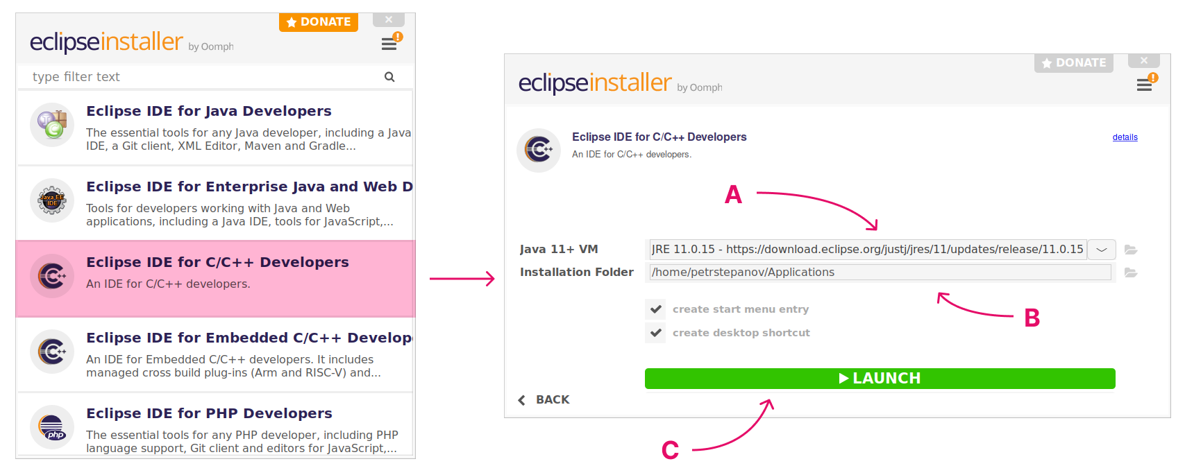
You can find (usually) outdated versions of QtCreator in your package manager, but I recommend to use the online installer, which then periodically checks for updates at program start. If you prefer not to open a user account with them, you can use the offline installer. While installing, I recommend to deactivate all Qt library options, newer CMake versions or Ninja. You will just need QtCreator.
Select your compiler Kit
Go to “Tools”, “Options”, “Kits”. Click for example on one of the auto-detected kits in the dialog. You can define your custom one, which will appear as “Manual” in the tree view. I recommend setting up a “Manual” kit, where “Qt version” is set to “None” (in case it was set), and in “CMake generator”, “Ninja” is changed to “Unix Makefiles” (if you are not in Windows). If you prefer to use the “Ninja” generator, make sure that it is installed in your system. Finally, click “Ok”.
Beware: in OSx, the “Tools”, “Options” menu is instead under “AppName”, “Preferences”.
Open a C++ CMake project
You can open any CMake project you have on your computer by clicking on “File”, “Open File or Project”. Find then the main folder where your project’s source code is located. Usually, there will be a “CMakeLists.txt” file in the main directory. Double-click then on this one, rather than in any other “CMakeLists.txt” that might appear in the subdirectories of this same project. If you prefer the command line, you can run directly as qtcreator my/folder/CMakeLists.txt &. If you installed QtCreator in a local folder, you might need to run something like: /opt/Qt/Tools/QtCreator/bin/qtcreator my/folder/CMakeLists.txt &.
If you rather use Makefiles, that’s also supported via the Import menu, by clicking on “File”, “New File or Project”, “Import Project”, “Import Existing Project”, “Choose”, and then select the source files you want to see in your tree (or just click on select all and deactivate those that are images, etc.). The Makefile will be automatically detected behind the scenes. You can edit the number of threads (-j) later on the project’s “Build settings”.
Let me load into QtCreator the simplest CMake example. After “Open File or Project”, a “Kit dialog” will apear. The button “Manage Kits” on the top left allows you to remember what compiler was associated with each kit (as explained above), click “Ok” to close. Select the “build kit” you prefer, and then click on “Details”. There, you can specify in what folder to build your program. Under “Tools”, “Options”, “Build”, “Default Properties” allows you to setup a default directory for your builds.
Once you click on “Configure Project”, CMake will be automatically run. In the “Projects” pane, you can tune any CMake flag as needed, as well as specify command line arguments when running. The “Build” hammer icon on the left compiles your project (make), and the “Run” play icon executes it.
You will not need to re-do all these configuration steps later on for this project, as QtCreator will store these settings in a file called “CMakeLists.txt.user” and recognize it automatically the next time you open the project.
The Power of F1
Let’s assume now that you have forgotten what class std::cout corresponds to. Luckily, Qt has an in-built (offline) help support system. For a first-time configuration, you will just need to download the “Help Book” of your library, in this case the std library from cppreference or via your package manager (sudo apt install cppreference-doc-en-qch). Then, in “Tools”, “Options”, “Help”, “Documentation”, you can add the downloaded (or /usr/share/ installed) “.qch” file.
Once this is set, you can either Ctrl+Click on your function or object to immediately go to the source code definition (file will open in another tab), or press F1, and the HTML documentation will appear on your right side without having to type / search anything online.

If you use and compile LLVM yourself, you can also get your Qt Help file as described here.
The ROOT framework also has a “.qch” Help Book available for download, thus you’ll be able to quickly consult any documentation using the F1 key, rather than searching online, which can be useful in case you are traveling and have no Internet access.

You can not only check the documentation with F1, but fully open the HTML reference guide by clicking on the big “Help” icon (left pane), as shown below.

Alternatively, you can also open the Help Books and search them using Qt Assistant. Linux apt packages are qt4-dev-tools or qt5-assistant, and the executables are assistant-qt4 and assistant, respectively. (qt6 version is not yet in the package manager.) You will have to add the .qch file to its database by going to “Edit”, “Preferences”, “Documentation”, “Add”.
And if you already use other IDEs or operating systems ? In addition to inline HTML searching, the building of the (ROOT) doxygen documentation can be configured to output a format that is compatible with MacOS - Xcode, Windows - VSstudio, or Eclipse. ROOT only provides for download the Qt help files (.qch) for the moment, but you can build the documentation yourself adapting those flags in the Doxyfile.
The Power of Clang
Grown over many years and standards, larger software projects have plenty of legacy code that is not as safe as the one someone would write today. Unsurprisingly, there are still some bugs here and there, and instabilities that haven’t been solved. Some of these bugs and potential style improvements can be detected thanks to the Clang-analyzer, which performs code analysis based on configurable settings.
QtCreator bundles perfectly with Clang-Analyzer, see left pane, “Debug” icon, then “Debugger” dropdown menu, “Clang-Tidy and Clazy”. It parses its output warnings and takes you directly to where the code needs to be changed.
In addition, it even lets you apply “fixits” by a mouse-click: if Clang knows how to correct the problem, he will change the code automatically for you.
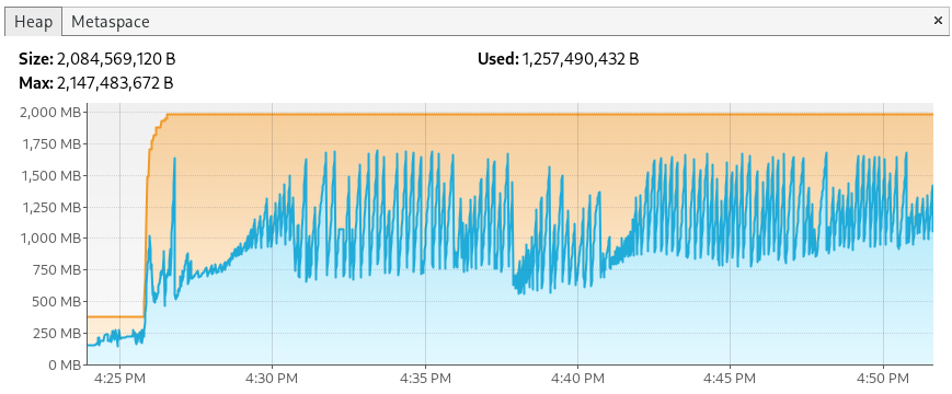
To give an example, analyzing the core of ROOT yields several diagnostics, and this can be quite useful for tracing in case you are seeing some memory leak when your application is deploying ROOT libraries:

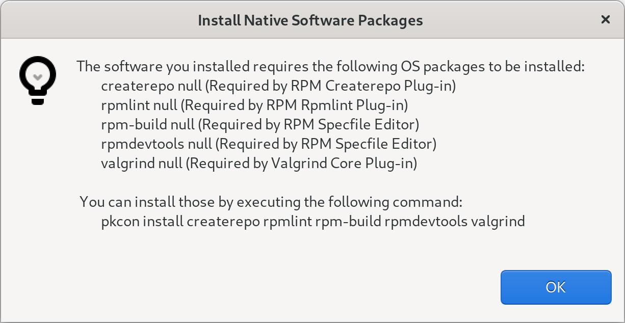
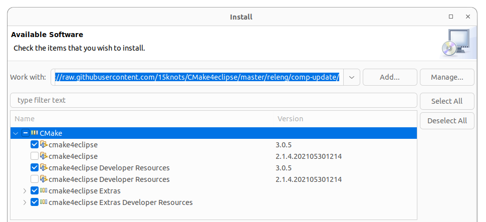
If, for example, you would like to modernize your code syntax to the latest C++ standard, you can configure the Clang settings in “Tools”, “Analyzer”, “Default checks”, and enable the modernize- option. For example, with a single click, you can change NULL to nullptr across your whole codebase.
Whether you like 4 spaces, 2 spaces, 1 tab, braces in the beginning or in the end… it does not matter what your taste is. What’s important is that you do not spend your valuable time on formatting things by hand. QtCreator can be helpful in this regard, too, if you activate the Beautifier plugin as well as install clang-format.
For example, let’s suppose you want to submit a pull request of one of your functions to ROOT, which has its own formatting guidelines. The easiest is to copy to your project the .clang-format configuration file from the repository or the website and then go to “Tools”, “Options”, “Beautifier”, “Clang Format”, and specify the file location. (Or if you are building ROOT itself using QtCreator, specify “File” in the dropdown menu, and it will auto-detect the one in the source tree).
You can also define a keyboard shortcut to format the file, by going to “Tools”, “Environment”, “Keyboard”, search for “format” and assign e.g. Ctrl+Alt+F.
Once that is configured, you can enable to auto-format your file when saving, or apply changes manually via Ctrl+Alt+F. Here a snippet before and after applying it:
int main(int argc, char* argv[])
{
int main(int argc, char *argv[]) {
git version control
For one of your projects, or even for the ROOT codebase, you might be using git for version control. QtCreator integrates seamlessly with the typical git commands, and can show you a visual diff of the current changes, as well as commit (Alt+G, Alt+C) and push your changes using its graphical interface, or pull the latest version from the remote repository.

Why bother with QtCreator when I am pro with emacs and vim?
You can get the best of both worlds by using the FakeVim mode or the emacs plugin. Just give it a try ;)
And if you just need column-editing, you don’t need any of those, QtCreator supports that natively.
CTests
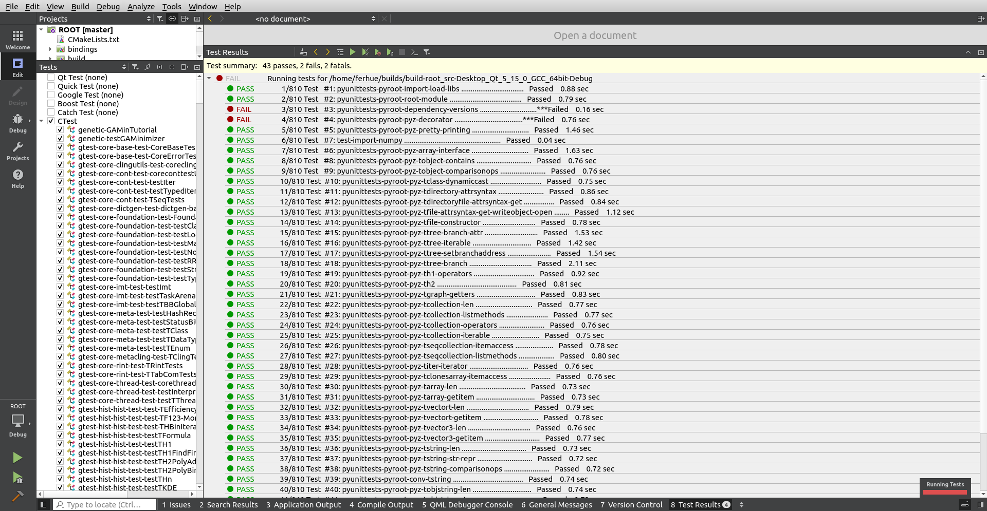
If you’ve built ROOT enabling the “testing” CMake flag, or if your project contains “CTests”, “Boost Tests”, etc. for ensuring that new changes you apply don’t break older functionality, QtCreator has a platform to visually run and check the results of all those tests. No need to scroll in a terminal to find which one failed.
Beware:
- Go first to “Tools”, “Options”, “Testing”, “General”, and adapt the total “Timeout” to allow running all tests at once.
- Be sure that the option “CTest” is active under “Active Frameworks” of that same menu.
To gild the lily
QtCreator lets you not only find compilation errors, but also documentation errors, by interfacing with the warnings issued by doxygen. This metawarning function can prove extremely useful for detecting outdated or incorrect documentation and going to the right spot in the source code in just one click, rather than diving through thousands of lines of output and tracing it manually.
To give it a try, take a look at building the ROOT documentation project. Follow these steps:
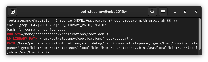
- Call first
source /path/to/ROOT/bin/thisroot.sh in the terminal and launch qtcreator from there. Alternatively, you can manually specify all the variables in the “Build” environment.
- Import the Makefile located in
root/documentation/doxygen into QtCreator, as explained above
- Click then on the “Build” icon.
Below a screenshot of the errors and the points in the source code found by just clicking on those issues.
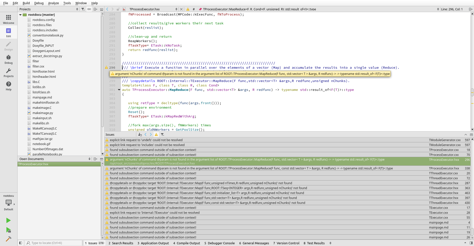
I’d suggest you to define a custom output parser to catch some doxygen warnings of “potential candidates” when there is an ambiguous matching in the signatures. To do this, go to “Tools”, “Options”, “Build&Run”, “Custom Output Parsers”, “Add”, and in “Warning”, specify the pattern (.*) at line (\d+) of file (.*) and order 3,2,1. “Apply”, “Ok”, and in the “Projects”, “Build Settings”, on the bottom, click on activate the newly defined “Parser”.
If you want even more verbose warnings about undocumented parameters, try setting WARN_NO_PARAMDOC to YES in the Doxyfile and EXTRACT_ALL to NO. This will account for many much more weak points of your documentation and let you pinpoint your efforts on the right spot. And while it can be burdensome to write all this extra missing documentation, QtCreator also simplifies the task by typing three magic characters on top a function. Then, it will autocomplete all the skeleton in doxygen format. Check first if “Tools”, “Text editor”, “Completion”, “Enable Doxygen blocks” is enabled.
Consider also enabling this spell-checking plugin for detecting typos in your documentation. This can be done by simply downloading the release file and unzipping into into your qtcreator folder. Then, under “Tools”, “Options”, “Spellchecker”, you can configure which dictionary or language(s) to use.

If you need to debug your ROOT scripts, or the ROOT library itself, I recommend building ROOT from its sources, but using the “Debug” flag.
Building ROOT in Debug Mode
To do this:
- Clone the ROOT git repository
- Open QtCreator
- “File”, “Open File or Project” and double click on the main “CMakeLists.txt” file.
- In the “Configure Project” dialog that will appear, you will be prompted to select which kit (compiler) you want to use for building.
- On the top left, you can click on “Manage Kits” to remember your different compiler choices. (See the kit configuration above). Click “Ok” to close.
- Click on the “checkbox” of the kit of choice for this build.
- Click then on “Details”. Activate the “Debug”, deactivate “Release”. The “Debug” mode will internally set the
CMAKE_BUILD_TYPE to Debug, as you would do from a command line.
- Specify also the folder where it will be built if you do not like the default choice. This can be set in the text box right from the “Debug” checkbox (while you are in the “Configure Project” - “your chosen Kit” dialog, “Details” dropdown unfolded).
- If you’ve already built ROOT using debug mode via your command line, then you can “import” your preexisting build, to not recompile it and save your time.
- Press then on the “Configure Project” button.
- On the left pane, press again on the “Projects” icon.
- At the bottom of the “Key” tree viewer, deactivate or activate submodules of ROOT as needed. This acts as passing
-Dmodule=ON via the command line.
- Consider enabling “testing” to run all ROOT tests.
- In the “Build steps” section, click on “Details”, and specify
-j8 on the “CMake arguments” or whatever other number, to speed up the build.
- On the left bottom pane, click on the “Build” (the big hammer) icon, and ROOT will be compiled.
- Once built, on the left, click on “Projects”, click on “your-Kit-name” on the left, under “Build & Run”, then on the “Run” small icon just below it, and under “Run configuration” on the right, select from the dropdown which executable you want to run. (The one selected by default might be “FileCheck”, click on it to change it).
- Under “Command line arguments”, specify what arguments you want to pass to this executable.
- Specify also the “Working directory”.
- If needed, activate the “Run in terminal” checkbox.
- You can then run it from the big “Play” icon on the left pane.
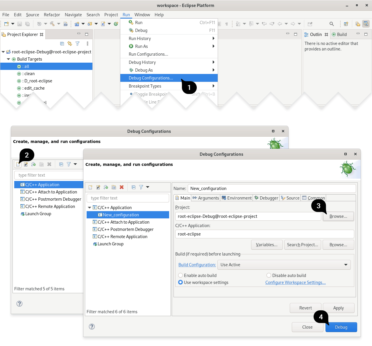
Debugging your ROOT scripts or executables with GDB
To debug your script, on the “Projects”, “Build & Run”, “Your-Kit-Name, “Run” settings, specify your executable right of “Run configuration” by clicking on the dropdown menu (your own standalone application, or root.exe) and specify your “Command line arguments”, e.g. -l -b as well as “Working directory”, e.g. the name of the script you want to run as well as their parameters. If you want to precompile instead of interpret with cling, consider using the debug flag g when passing the command line argument (yourScript.C+g)
Click then on the “Play-Bug” icon on the left, and your script will run in “Debug” mode. Breakpoints can be set interactively on your code. F5 will pause or resume your process, as well as show you a workspace of the active variables and threads. For example, specify as “Command line arguments” -l -b hsimple.C+ -q and as working directory your-root-folder/tutorials. Open this file within QtCreator, and click on the left of the line numbers, and then click on the “Play-Bug” icon on the left, the script will execute and pause when it reaches that point. You can then perform step-by-step execution using the three little arrow icons right from the “Debugger” dropdown menu. You can hover your mouse over them and a tooltip will show their function.
Below a screenshot of another example, while debugging a deadlock in the TThread class.

Side note: if at some point, your ROOT script gets very complex long, I recommend instead to use a standalone C++ application using CMake, and link the ROOT libraries easily to it, as explained here.
Memory error detection
To check for memory leaks and corruption, QtCreator offers a seamless integration with valgrind (or heob on Windows), making the backtrace of your errors fully interactive. To run it, press on the big “Debug button” on the left. Then, on the dropdown menu, change from “Debugger” to “Memcheck” and click on the small play button.
If you need extra arguments for valgrind, you will need to specify those under “Tools”, “Options”, “Analyzer”, “Valgrind”.
There, I also recommend to click on “Add”, “etc/valgrind-root.supp” from your cloned repository, to suppress spurious warnings.
The resulting warnings can be easily clicked to bring you to the right spot in your code, or in the ROOT codebase, where the issue is arising from.
Often, you will also find helpful to run the static Clang-analyzer, which is able to detect many unsafe parts of your code that might be leading to memory leaks. It’s in the same dropdown menu, under “Clang-Tidy and Clazy”.
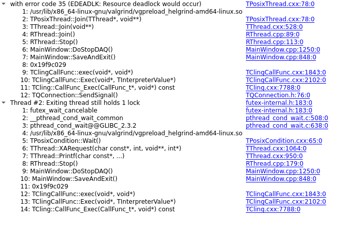
Data race detection
First, I recommend to click on “Tools”, “Options”, “Analyzer”, “Valgrind”, “Add”, “etc/valgrind-root.supp” from your git repository. Then, on the dropdown menu, change from “Debugger” to “Memcheck” and click on the small play button.
Helgrind cannot be run yet directly from QtCreator. The workaround is to run root.exe or your own executable from your command line, with the flags --tool=helgrind --xml=yes --xml-file=yourfile.xml. Then, you can “load” the result using the small “open” button right from the dropdown menu. The parsing tool works great and takes you the relevant location in your code.
In case you want to optimize the performance of your code, you can select from the debugger dropdown menu between “Callgrind” or the Performance Analyzer. If you install and use callgrind, consider installing also kcachegrind for visualization.
Other approaches
There are other tricks to boost your development in a way that’s integrated with your IDE. For example:
- If you use a standalone application that uses ROOT libraries and graphical interface, but not it’s terminal, you might want to check the TGCommandPlugin window. With it, you can nicely interact with your internal C++ classes while your program is executing, without having to build in “Debug” mode, which has sometimes downsides due to its slow performance. To make ROOT aware of your C++ object, you need to call within your program:
gROOT->ProcessLine(
    static_cast<TString>(
        "MyClassType* const fMyInstance = reinterpret_cast<MyClasstype*>(") +
    dynamic_cast<std::ostringstream &&>(std::ostringstream("") << fMyInstance)
        .str() +
    ");");
And then, of course, creating a TGCommandPlugin window. From there, typing fMyInstance->MyMethod() will execute binary code interactively.
-
This VS Studio plugin allows for a nice integration of a ROOT file browser. Maybe it will come at some point for QtCreator, too.
- Interfaces between Cling and Qt have been attempted before.
Quick recipe Summary
- Optional: install
valgrind, callgrind, kcachegrind.
- Install QtCreator deactivating all extra options.
- Download std Help Book from cppreference or package manager (
sudo apt install cppreference-doc-en-qch).
- Download ROOT Help Book.
- Add both “.qch” files via “Tools”, “Options”, “Help”, “Documentation”.
- “Tools”, “Options”, “Analyzer”, “Default checks”, configure as needed.
- Install the Beautifier plugin, potentially download the ROOT one to store in your own project.
- “Tools”, “Options”, “Beautifier”, “Clang”, “Use predefined style”, “File”
- If you enable “testing” flag in CMake, adapt “Timeout” in “Tools”, “Options”, “Testing”.
- Be sure that the option “CTest” is active under “Active Frameworks” of that same menu.
- Optional: Check that “Tools”, “Kits”, you have selected the compiler you want, as well as “CMake generator”. If you use Ninja, make sure it’s installed.
- Optional: Check that “Tools”, “Text editor”, “Completion”, “Enable Doxygen blocks” is enabled.
- Optional: Under “Tools”, “Options”, “Build & Run”, “Custom Output Parsers”, “Add”, “Warning”, specify the pattern
(.*) at line (\d+) of file (.*) and order 3,2,1. “Apply”, “Ok”. Activate it under “Projects”, “Build Settings”, on the bottom.
- Optional: Install a spellchecker plugin by unzipping the release file into your QtCreator installation folder. Configure then your dictionary under “Tools”, “Options”, “Spellchecker”.
- Clone the ROOT git repository and open main “CMakeLists.txt” with QtCreator.
- Optional: configure your default’s “Kit” build directory to e.g.
~/builds/.
- Specify
-j8 on “Projects”, “Build & Run”, “Kit-name”, “Build”, “Build Steps”, and root.exe as your executable in the run settings.
- Optional: also specify the “Working directory”.
- “Tools”, “Options”, “Analyzer”, “Valgrind”, “Add”, “etc/valgrind-root.supp” and “etc/helgrind-root.supp” from your cloned repository.
Setting up all this platform requires some initial effort, but once it is running, it will smooth your development and bug hunting, and once you’ve get used to it, you will find it much more tiring to program without it ;) .
Fernando Hueso-González
IFIC - Instituto de Física Corpuscular (CSIC / Universitat de València)
]]>