
 This macro shows in detail the use of the quadratic programming package quadp .
Running this macro :
or
.L portFolio.C+; portfolio()
Let's first review what we exactly mean by "quadratic programming" :
We want to minimize the following objective function :
\( c^T x + ( 1/2 ) x^T Q x \) wrt. the vector \( x \)
\( c \) is a vector and \( Q \) a symmetric positive definite matrix
You might wonder what is so special about this objective which is quadratic in the unknowns, that can not be done by Minuit/Fumili . Well, we have in addition the following boundary conditions on \( x \):
\[ A x = b \\ clo \le C x \le cup \\ xlo \le x \le xup \]
where A and C are arbitrary matrices and the rest are vectors
Not all these constraints have to be defined . Our example will only use \( xlo \), \( A \) and \( b \) Still, this could be handled by a general non-linear minimizer like Minuit by introducing so-called "slack" variables . However, quadp is tailored to objective functions not more complex than being quadratic . This allows usage of solving techniques which are even stable for problems involving for instance 500 variables, 100 inequality conditions and 50 equality conditions .
Enough said about quadratic programming, let's return to our example . Suppose, after a long day of doing physics, you have a look at your investments and realize that an early retirement is not possible, given the returns of your stocks . So what now ? ROOT to the rescue ...
In 1990 Harry Markowitz was awarded the Nobel prize for economics: " his work provided new tools
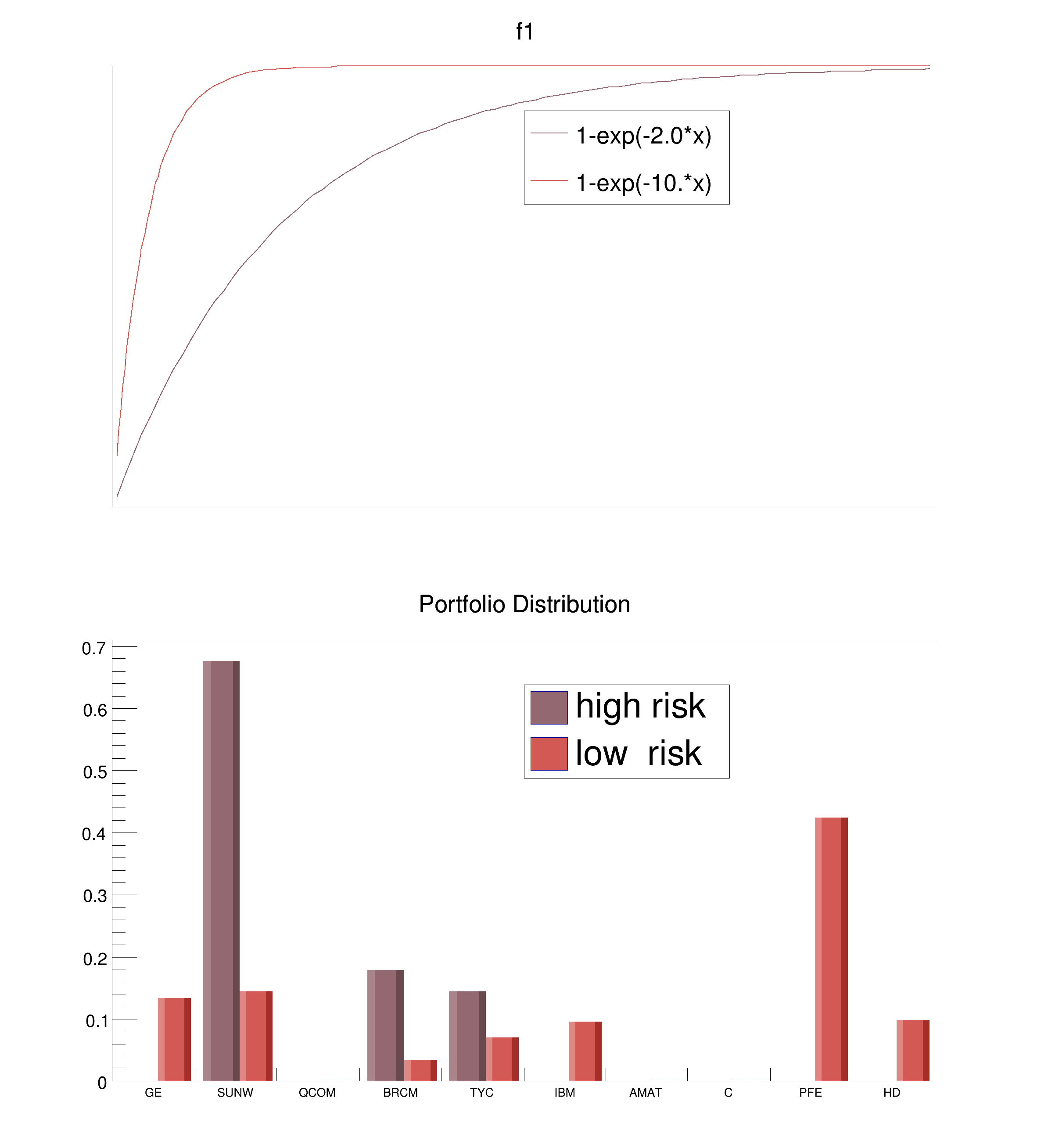
for weighing the risks and rewards of different investments and for valuing corporate stocks and bonds" . In plain English, he developed the tools to balance greed and fear, we want the maximum return with the minimum amount of risk. Our stock portfolio should be at the "Efficient Frontier". To quantify better the risk we are willing to take, we define a utility function \( U(x) \). It describes as a function of our total assets \( x \), our "satisfaction" . A common choice is \( 1-exp(-k*x) \) (the reason for the exponent will be clear later) . The parameter \( k \) is the risk-aversion factor . For small values of \( k \) the satisfaction is small for small values of \( x \); by increasing \( x \) the satisfaction can still be increased significantly . For large values of \( k \), \( U(x) \) increases rapidly to 1, there is no increase in satisfaction for additional dollars earned .
In summary :
- small \( k \) ==> risk-loving investor
- large \( k \) ==> risk-averse investor
Suppose we have for nrStocks the historical daily returns \( r = closing_price(n) - closing_price(n-1) \). Define a vector \( x \) of length of \( nrStocks \), which contains the fraction of our money invested in each stock . We can calculate the average daily return \( z \) of our portfolio and its variance using the portfolio covariance Covar :
\( z = r^T x \) and \( var = x^T Covar x \)
Assuming that the daily returns have a Normal distribution, \( N(x) \), so will \( z \) with mean \( r^T x \) and variance \( x^T Covar x \)
The expected value of the utility function is :
\[ E(u(x)) = Int (1-exp(-k*x) N(x) dx \\ = 1-exp(-k (r^T x - 0.5 k x^T Covar x) ) \\ \]
Its value is maximised by maximising \( r^T x -0.5 k x^T Covar x \) under the condition \( sum (x_i) = 1 \), meaning we want all our money invested and \( x_i \ge 0 \), we can not "short" a stock
For 10 stocks we got the historical daily data for Sep-2000 to Jun-2004:
- GE : General Electric Co
- SUNW : Sun Microsystems Inc
- QCOM : Qualcomm Inc
- BRCM : Broadcom Corp
- TYC : Tyco International Ltd
- IBM : International Business Machines Corp
- AMAT : Applied Materials Inc
- C : Citigroup Inc
- PFE : Pfizer Inc
- HD : Home Depot Inc
We calculate the optimal portfolio for 2.0 and 10.0 .
Food for thought :
- We assumed that the stock returns have a Normal distribution . Check this assumption by histogramming the stock returns !
- We used for the expected return in the objective function, the flat average over a time period . Investment firms will put significant resources in improving the return prediction .
- If you want to trade significant number of shares, several other considerations have to be taken into account :
- If you are going to buy, you will drive the price up (so-called "slippage") . This can be taken into account by adding terms to the objective (Google for "slippage optimization")
- FTC regulations might have to be added to the inequality constraints
- Investment firms do not want to be exposed to the "market" as defined by a broad index like the S&P and "hedge" this exposure away . A perfect hedge this can be added as an equality constrain, otherwise add an inequality constrain .
Processing /mnt/build/workspace/root-makedoc-v614/rootspi/rdoc/src/v6-14-00-patches/tutorials/quadp/portfolio.C...
stock daily daily w1 w2
symb return sdv
GE : 1.001 0.022 0.000 0.134
SUNW : 1.004 0.047 0.676 0.145
QCOM : 1.001 0.039 0.000 0.000
BRCM : 1.003 0.056 0.179 0.035
TYC : 1.001 0.042 0.145 0.069
IBM : 1.001 0.023 0.000 0.096
AMAT : 1.001 0.040 0.000 0.000
C : 1.000 0.023 0.000 0.000
PFE : 1.000 0.019 0.000 0.424
HD : 1.001 0.029 0.000 0.098
const Int_t nrStocks = 10;
static const Char_t *stocks[] =
{"GE","SUNW","QCOM","BRCM","TYC","IBM","AMAT","C","PFE","HD"};
class TStockDaily {
public:
TStockDaily() {
fDate = fVol = fOpen = fHigh = fLow = fClose = fCloseAdj = 0;
}
virtual ~TStockDaily() {}
};
}
{
TStockDaily *data = 0;
for (
Int_t i = 0; i < nrEntries; i++) {
if (data->fDate >= sDay && data->fDate <= eDay)
closeAdj[i] = data->fCloseAdj/100.;
}
for (
Int_t i = 1; i < nrEntries; i++)
(*r)[i-1] = closeAdj[i]/closeAdj[i-1];
}
#ifndef __MAKECINT__
{
const Int_t nrVar = nrStocks;
const Int_t nrInEqual = 0;
TQpDataDens *prob = (
TQpDataDens *)qp->
MakeData(c,Q,xlo,ixlo,xup,ixup,
A,b,C,clo,iclo,cup,icup);
delete qp;
delete prob;
delete vars;
delete resid;
delete s;
if (status != 0) {
cout << "Could not solve this problem." <<endl;
}
return weight;
}
#endif
void portfolio()
{
const Int_t sDay = 20000809;
const Int_t eDay = 20040602;
const char *fname = "stock.root";
} else {
printf("accessing %s file from http://root.cern.ch/files\n",fname);
}
if (!f) return;
for (
Int_t i = 0; i < nrStocks; i++) {
data[i] = StockReturn(f,symbol,sDay,eDay);
}
for (
Int_t i = 0; i < nrStocks; i++)
r[i] = data[i].GetSum()/nrData;
for (
Int_t i = 0; i < nrStocks; i++) {
for (
Int_t j = 0; j <= i; j++) {
for (
Int_t k = 0; k < nrData; k++) {
sum += (data[i][k] - r[i]) * (data[j][k] - r[j]);
}
Covar(i,j) = Covar(j,i) = sum/nrData;
}
}
const TVectorD weight1 = OptimalInvest(2.0,r,Covar);
const TVectorD weight2 = OptimalInvest(10.,r,Covar);
cout << "stock daily daily w1 w2" <<endl;
cout << "symb return sdv " <<endl;
for (
Int_t i = 0; i < nrStocks; i++)
printf(
"%s\t: %.3f %.3f %.3f %.3f\n",stocks[i],r[i],
TMath::Sqrt(Covar[i][i]),weight1[i],weight2[i]);
TCanvas *c1 =
new TCanvas(
"c1",
"Portfolio Optimizations",10,10,800,900);
TF1 *f1 =
new TF1(
"f1",RiskProfile,0,2.5,1);
TF1 *f2 =
new TF1(
"f2",RiskProfile,0,2.5,1);
legend1->
AddEntry(f1,
"1-exp(-2.0*x)",
"l");
legend1->
AddEntry(f2,
"1-exp(-10.*x)",
"l");
TH1F *h1 =
new TH1F(
"h1",
"Portfolio Distribution",nrStocks,0,0);
TH1F *h2 =
new TH1F(
"h2",
"Portfolio Distribution",nrStocks,0,0);
for (
Int_t i = 0; i < nrStocks; i++) {
h1->
Fill(stocks[i],weight1[i]);
h2->
Fill(stocks[i],weight2[i]);
}
h2->
Draw(
"BAR2SAME HIST");
}
- Author
- Eddy Offermann
Definition in file portfolio.C.

 ROOT 6.14/05 - Reference Guide Generated on Fri Nov 2 2018 10:58:50 (GVA Time) using Doxygen 1.8.13.