Logo ROOT   6.14/05
Reference Guide
HybridStandardForm.C File Reference

Detailed Description

View in nbviewer Open in SWAN A hypothesis testing example based on number counting with background uncertainty.

A hypothesis testing example based on number counting with background uncertainty.

NOTE: This example is like HybridInstructional, but the model is more clearly generalizable to an analysis with shapes. There is a lot of flexibility for how one models a problem in RooFit/RooStats. Models come in a few common forms:

Here we convert the number counting form into the standard form by introducing a dummy discriminating variable m with a uniform distribution.

This example:

The basic setup here is that a main measurement has observed x events with an expectation of s+b. One can choose an ad hoc prior for the uncertainty on b, or try to base it on an auxiliary measurement. In this case, the auxiliary measurement (aka control measurement, sideband) is another counting experiment with measurement y and expectation tau*b. With an 'original prior' on b, called \( \eta(b) \) then one can obtain a posterior from the auxiliary measurement \( \pi(b) = \eta(b) * Pois(y|tau*b) \). This is a principled choice for a prior on b in the main measurement of x, which can then be treated in a hybrid Bayesian/Frequentist way. Additionally, one can try to treat the two measurements simultaneously, which is detailed in Part 6 of the tutorial.

This tutorial is related to the FourBin.C tutorial in the modeling, but focuses on hypothesis testing instead of interval estimation.

More background on this 'prototype problem' can be found in the following papers:

pict1_HybridStandardForm.C.png
Processing /mnt/build/workspace/root-makedoc-v614/rootspi/rdoc/src/v6-14-00-patches/tutorials/roostats/HybridStandardForm.C...
RooFit v3.60 -- Developed by Wouter Verkerke and David Kirkby
Copyright (C) 2000-2013 NIKHEF, University of California & Stanford University
All rights reserved, please read http://roofit.sourceforge.net/license.txt
-----------------------------------------
Part 3
Z_Bi p-value (analytic): 0.00094165
Z_Bi significance (analytic): 3.10804
Real time 0:00:00, CP time 0.020
[#0] WARNING:Eval -- RooStatsUtils::MakeNuisancePdf - no constraints found on nuisance parameters in the input model
[#0] WARNING:Eval -- RooStatsUtils::MakeNuisancePdf - no constraints found on nuisance parameters in the input model
-----------------------------------------
Part 4
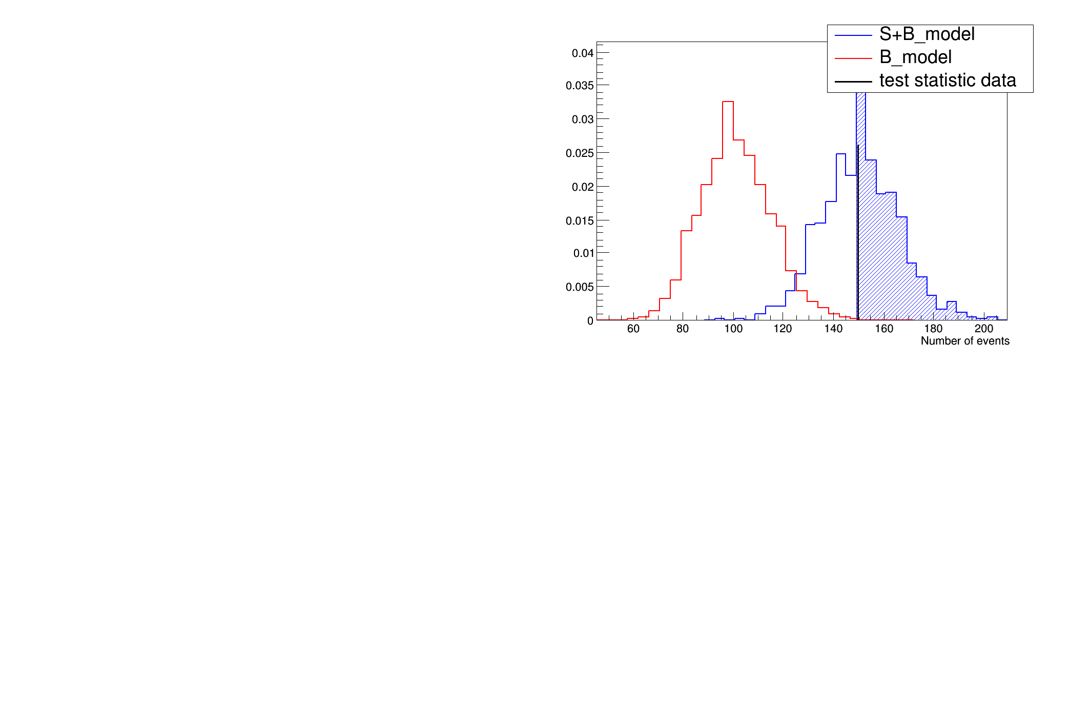
Results HypoTestCalculator_result:
- Null p-value = 0.0009 +/- 0.000173127
- Significance = 3.12139 +/- 0.0566416 sigma
- Number of Alt toys: 1000
- Number of Null toys: 30000
- Test statistic evaluated on data: 150
- CL_b: 0.0009 +/- 0.000173127
- CL_s+b: 0.533 +/- 0.0157769
- CL_s: 592.222 +/- 115.263
Real time 0:00:51, CP time 51.070
#include "RooGlobalFunc.h"
#include "RooRealVar.h"
#include "RooProdPdf.h"
#include "RooWorkspace.h"
#include "RooDataSet.h"
#include "RooDataHist.h"
#include "TCanvas.h"
#include "TStopwatch.h"
#include "TH1.h"
#include "RooPlot.h"
#include "RooMsgService.h"
using namespace RooFit;
using namespace RooStats;
//-------------------------------------------------------
// A New Test Statistic Class for this example.
// It simply returns the sum of the values in a particular
// column of a dataset.
// You can ignore this class and focus on the macro below
class BinCountTestStat : public TestStatistic {
public:
BinCountTestStat(void) : fColumnName("tmp") {}
BinCountTestStat(string columnName) : fColumnName(columnName) {}
virtual Double_t Evaluate(RooAbsData& data, RooArgSet& /*nullPOI*/) {
// This is the main method in the interface
Double_t value = 0.0;
for(int i=0; i < data.numEntries(); i++) {
value += data.get(i)->getRealValue(fColumnName.c_str());
}
return value;
}
virtual const TString GetVarName() const { return fColumnName; }
private:
string fColumnName;
protected:
ClassDef(BinCountTestStat,1)
};
ClassImp(BinCountTestStat)
//-----------------------------
// The Actual Tutorial Macro
//-----------------------------
void HybridStandardForm() {
// This tutorial has 6 parts
// Table of Contents
// Setup
// 1. Make the model for the 'prototype problem'
// Special cases
// 2. NOT RELEVANT HERE
// 3. Use RooStats analytic solution for this problem
// RooStats HybridCalculator -- can be generalized
// 4. RooStats ToyMC version of 2. & 3.
// 5. RooStats ToyMC with an equivalent test statistic
// 6. RooStats ToyMC with simultaneous control & main measurement
// Part 4 takes ~4 min without PROOF.
// Part 5 takes about ~2 min with PROOF on 4 cores.
// Of course, everything looks nicer with more toys, which takes longer.
t.Start();
TCanvas *c = new TCanvas;
c->Divide(2,2);
//-----------------------------------------------------
// P A R T 1 : D I R E C T I N T E G R A T I O N
// ====================================================
// Make model for prototype on/off problem
// Pois(x | s+b) * Pois(y | tau b )
// for Z_Gamma, use uniform prior on b.
RooWorkspace* w = new RooWorkspace("w");
// replace the pdf in 'number counting form'
//w->factory("Poisson::px(x[150,0,500],sum::splusb(s[0,0,100],b[100,0,300]))");
// with one in standard form. Now x is encoded in event count
w->factory("Uniform::f(m[0,1])");//m is a dummy discriminating variable
w->factory("ExtendPdf::px(f,sum::splusb(s[0,0,100],b[100,0,300]))");
w->factory("Poisson::py(y[100,0,500],prod::taub(tau[1.],b))");
w->factory("PROD::model(px,py)");
w->factory("Uniform::prior_b(b)");
// We will control the output level in a few places to avoid
// verbose progress messages. We start by keeping track
// of the current threshold on messages.
// Use PROOF-lite on multi-core machines
ProofConfig* pc = NULL;
// uncomment below if you want to use PROOF
pc = new ProofConfig(*w, 4, "workers=4", kFALSE); // machine with 4 cores
// pc = new ProofConfig(*w, 2, "workers=2", kFALSE); // machine with 2 cores
//-----------------------------------------------
// P A R T 3 : A N A L Y T I C R E S U L T
// ==============================================
// In this special case, the integrals are known analytically
// and they are implemented in RooStats::NumberCountingUtils
// analytic Z_Bi
double p_Bi = NumberCountingUtils::BinomialWithTauObsP(150, 100, 1);
double Z_Bi = NumberCountingUtils::BinomialWithTauObsZ(150, 100, 1);
cout << "-----------------------------------------"<<endl;
cout << "Part 3" << endl;
std::cout << "Z_Bi p-value (analytic): " << p_Bi << std::endl;
std::cout << "Z_Bi significance (analytic): " << Z_Bi << std::endl;
t.Stop(); t.Print(); t.Reset(); t.Start();
//--------------------------------------------------------------
// P A R T 4 : U S I N G H Y B R I D C A L C U L A T O R
// ==============================================================
// Now we demonstrate the RooStats HybridCalculator.
//
// Like all RooStats calculators it needs the data and a ModelConfig
// for the relevant hypotheses. Since we are doing hypothesis testing
// we need a ModelConfig for the null (background only) and the alternate
// (signal+background) hypotheses. We also need to specify the PDF,
// the parameters of interest, and the observables. Furthermore, since
// the parameter of interest is floating, we need to specify which values
// of the parameter corresponds to the null and alternate (eg. s=0 and s=50)
//
// define some sets of variables obs={x} and poi={s}
// note here, x is the only observable in the main measurement
// and y is treated as a separate measurement, which is used
// to produce the prior that will be used in this calculation
// to randomize the nuisance parameters.
w->defineSet("obs","m");
w->defineSet("poi","s");
// create a toy dataset with the x=150
// RooDataSet *data = new RooDataSet("d", "d", *w->set("obs"));
// data->add(*w->set("obs"));
RooDataSet* data = w->pdf("px")->generate(*w->set("obs"),150);
// Part 3a : Setup ModelConfigs
//-------------------------------------------------------
// create the null (background-only) ModelConfig with s=0
ModelConfig b_model("B_model", w);
b_model.SetPdf(*w->pdf("px"));
b_model.SetObservables(*w->set("obs"));
b_model.SetParametersOfInterest(*w->set("poi"));
w->var("s")->setVal(0.0); // important!
b_model.SetSnapshot(*w->set("poi"));
// create the alternate (signal+background) ModelConfig with s=50
ModelConfig sb_model("S+B_model", w);
sb_model.SetPdf(*w->pdf("px"));
sb_model.SetObservables(*w->set("obs"));
sb_model.SetParametersOfInterest(*w->set("poi"));
w->var("s")->setVal(50.0); // important!
sb_model.SetSnapshot(*w->set("poi"));
// Part 3b : Choose Test Statistic
//--------------------------------------------------------------
// To make an equivalent calculation we need to use x as the test
// statistic. This is not a built-in test statistic in RooStats
// so we define it above. The new class inherits from the
// RooStats::TestStatistic interface, and simply returns the value
// of x in the dataset.
NumEventsTestStat eventCount(*w->pdf("px"));
// Part 3c : Define Prior used to randomize nuisance parameters
//-------------------------------------------------------------
//
// The prior used for the hybrid calculator is the posterior
// from the auxiliary measurement y. The model for the aux.
// measurement is Pois(y|tau*b), thus the likelihood function
// is proportional to (has the form of) a Gamma distribution.
// if the 'original prior' $\eta(b)$ is uniform, then from
// Bayes's theorem we have the posterior:
// $\pi(b) = Pois(y|tau*b) * \eta(b)$
// If $\eta(b)$ is flat, then we arrive at a Gamma distribution.
// Since RooFit will normalize the PDF we can actually supply
// py=Pois(y,tau*b) that will be equivalent to multiplying by a uniform.
//
// Alternatively, we could explicitly use a gamma distribution:
//
// `w->factory("Gamma::gamma(b,sum::temp(y,1),1,0)");`
//
// or we can use some other ad hoc prior that do not naturally
// follow from the known form of the auxiliary measurement.
// The common choice is the equivalent Gaussian:
w->factory("Gaussian::gauss_prior(b,y, expr::sqrty('sqrt(y)',y))");
// this corresponds to the "Z_N" calculation.
//
// or one could use the analogous log-normal prior
w->factory("Lognormal::lognorm_prior(b,y, expr::kappa('1+1./sqrt(y)',y))");
//
// Ideally, the HybridCalculator would be able to inspect the full
// model Pois(x | s+b) * Pois(y | tau b ) and be given the original
// prior $\eta(b)$ to form $\pi(b) = Pois(y|tau*b) * \eta(b)$.
// This is not yet implemented because in the general case
// it is not easy to identify the terms in the PDF that correspond
// to the auxiliary measurement. So for now, it must be set
// explicitly with:
// - ForcePriorNuisanceNull()
// - ForcePriorNuisanceAlt()
// the name "ForcePriorNuisance" was chosen because we anticipate
// this to be auto-detected, but will leave the option open
// to force to a different prior for the nuisance parameters.
// Part 3d : Construct and configure the HybridCalculator
//-------------------------------------------------------
HybridCalculator hc1(*data, sb_model, b_model);
ToyMCSampler *toymcs1 = (ToyMCSampler*)hc1.GetTestStatSampler();
// toymcs1->SetNEventsPerToy(1); // because the model is in number counting form
toymcs1->SetTestStatistic(&eventCount); // set the test statistic
// toymcs1->SetGenerateBinned();
hc1.SetToys(30000,1000);
hc1.ForcePriorNuisanceAlt(*w->pdf("py"));
hc1.ForcePriorNuisanceNull(*w->pdf("py"));
// if you wanted to use the ad hoc Gaussian prior instead
// ~~~
// hc1.ForcePriorNuisanceAlt(*w->pdf("gauss_prior"));
// hc1.ForcePriorNuisanceNull(*w->pdf("gauss_prior"));
// ~~~
// if you wanted to use the ad hoc log-normal prior instead
// ~~~
// hc1.ForcePriorNuisanceAlt(*w->pdf("lognorm_prior"));
// hc1.ForcePriorNuisanceNull(*w->pdf("lognorm_prior"));
// ~~~
// enable proof
// proof not enabled for this test statistic
// if(pc) toymcs1->SetProofConfig(pc);
// these lines save current msg level and then kill any messages below ERROR
// Get the result
HypoTestResult *r1 = hc1.GetHypoTest();
RooMsgService::instance().setGlobalKillBelow(msglevel); // set it back
cout << "-----------------------------------------"<<endl;
cout << "Part 4" << endl;
r1->Print();
t.Stop(); t.Print(); t.Reset(); t.Start();
c->cd(2);
HypoTestPlot *p1 = new HypoTestPlot(*r1,30); // 30 bins, TS is discrete
p1->Draw();
return; // keep the running time sort by default
//-------------------------------------------------------------------------
// # P A R T 5 : U S I N G H Y B R I D C A L C U L A T O R W I T H
// # A N A L T E R N A T I V E T E S T S T A T I S T I C
//
// A likelihood ratio test statistics should be 1-to-1 with the count x
// when the value of b is fixed in the likelihood. This is implemented
// by the SimpleLikelihoodRatioTestStat
SimpleLikelihoodRatioTestStat slrts(*b_model.GetPdf(),*sb_model.GetPdf());
slrts.SetNullParameters(*b_model.GetSnapshot());
slrts.SetAltParameters(*sb_model.GetSnapshot());
// HYBRID CALCULATOR
HybridCalculator hc2(*data, sb_model, b_model);
ToyMCSampler *toymcs2 = (ToyMCSampler*)hc2.GetTestStatSampler();
// toymcs2->SetNEventsPerToy(1);
toymcs2->SetTestStatistic(&slrts);
// toymcs2->SetGenerateBinned();
hc2.SetToys(20000,1000);
hc2.ForcePriorNuisanceAlt(*w->pdf("py"));
hc2.ForcePriorNuisanceNull(*w->pdf("py"));
// if you wanted to use the ad hoc Gaussian prior instead
// ~~~
// hc2.ForcePriorNuisanceAlt(*w->pdf("gauss_prior"));
// hc2.ForcePriorNuisanceNull(*w->pdf("gauss_prior"));
// ~~~
// if you wanted to use the ad hoc log-normal prior instead
// ~~~
// hc2.ForcePriorNuisanceAlt(*w->pdf("lognorm_prior"));
// hc2.ForcePriorNuisanceNull(*w->pdf("lognorm_prior"));
// ~~~
// enable proof
if(pc) toymcs2->SetProofConfig(pc);
// these lines save current msg level and then kill any messages below ERROR
// Get the result
HypoTestResult *r2 = hc2.GetHypoTest();
cout << "-----------------------------------------"<<endl;
cout << "Part 5" << endl;
r2->Print();
t.Stop(); t.Print(); t.Reset(); t.Start();
c->cd(3);
HypoTestPlot *p2 = new HypoTestPlot(*r2,30); // 30 bins
p2->Draw();
return; // so standard tutorial runs faster
//---------------------------------------------
// OUTPUT W/O PROOF (2.66 GHz Intel Core i7)
// ============================================
// -----------------------------------------
// Part 3
// Z_Bi p-value (analytic): 0.00094165
// Z_Bi significance (analytic): 3.10804
// Real time 0:00:00, CP time 0.610
// Results HybridCalculator_result:
// - Null p-value = 0.00103333 +/- 0.000179406
// - Significance = 3.08048 sigma
// - Number of S+B toys: 1000
// - Number of B toys: 30000
// - Test statistic evaluated on data: 150
// - CL_b: 0.998967 +/- 0.000185496
// - CL_s+b: 0.495 +/- 0.0158106
// - CL_s: 0.495512 +/- 0.0158272
// Real time 0:04:43, CP time 283.780
// With PROOF
// -----------------------------------------
// Part 5
// Results HybridCalculator_result:
// - Null p-value = 0.00105 +/- 0.000206022
// - Significance = 3.07571 sigma
// - Number of S+B toys: 1000
// - Number of B toys: 20000
// - Test statistic evaluated on data: 10.8198
// - CL_b: 0.99895 +/- 0.000229008
// - CL_s+b: 0.491 +/- 0.0158088
// - CL_s: 0.491516 +/- 0.0158258
// Real time 0:02:22, CP time 0.990
//-------------------------------------------------------
// Comparison
//-------------------------------------------------------
// LEPStatToolsForLHC
// https://plone4.fnal.gov:4430/P0/phystat/packages/0703002
// Uses Gaussian prior
// CL_b = 6.218476e-04, Significance = 3.228665 sigma
//
//-------------------------------------------------------
// Comparison
//-------------------------------------------------------
// Asymptotic
// From the value of the profile likelihood ratio (5.0338)
// The significance can be estimated using Wilks's theorem
// significance = sqrt(2*profileLR) = 3.1729 sigma
}
Authors
Kyle Cranmer, Wouter Verkerke, and Sven Kreiss

Definition in file HybridStandardForm.C.