FFT.C File Reference

Detailed Description

This tutorial illustrates the Fast Fourier Transforms interface in ROOT.

FFT transform types provided in ROOT:

• "C2CFORWARD" - a complex input/output discrete Fourier transform (DFT) in one or more dimensions, -1 in the exponent
• "C2CBACKWARD"- a complex input/output discrete Fourier transform (DFT) in one or more dimensions, +1 in the exponent
• "R2C" - a real-input/complex-output discrete Fourier transform (DFT) in one or more dimensions,
• "C2R" - inverse transforms to "R2C", taking complex input (storing the non-redundant half of a logically Hermitian array) to real output
• "R2HC" - a real-input DFT with output in "halfcomplex" format, i.e. real and imaginary parts for a transform of size n stored as r0, r1, r2, ..., rn/2, i(n+1)/2-1, ..., i2, i1
• "HC2R" - computes the reverse of FFTW_R2HC, above
• "DHT" - computes a discrete Hartley transform

Sine/cosine transforms:

• DCT-I (REDFT00 in FFTW3 notation)
• DCT-II (REDFT10 in FFTW3 notation)
• DCT-III(REDFT01 in FFTW3 notation)
• DCT-IV (REDFT11 in FFTW3 notation)
• DST-I (RODFT00 in FFTW3 notation)
• DST-II (RODFT10 in FFTW3 notation)
• DST-III(RODFT01 in FFTW3 notation)
• DST-IV (RODFT11 in FFTW3 notation)

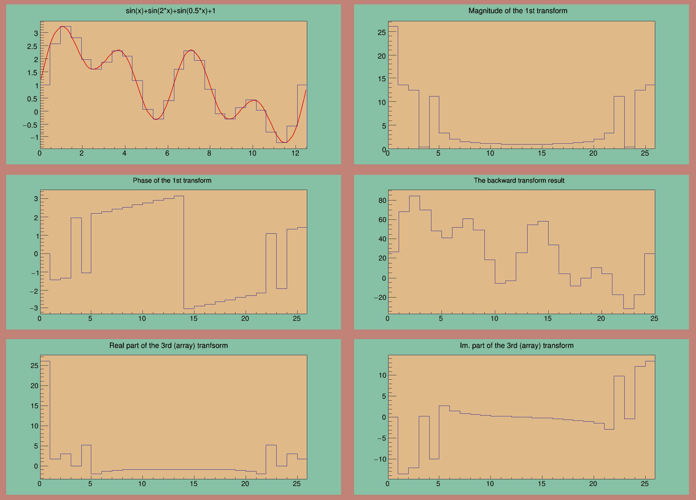
First part of the tutorial shows how to transform the histograms Second part shows how to transform the data arrays directly

Processing /mnt/build/workspace/root-makedoc-v614/rootspi/rdoc/src/v6-14-00-patches/tutorials/fft/FFT.C...
1st transform: DC component: 26.000000
1st transform: Nyquist harmonic: -0.932840
2nd transform: DC component: 29.000000
2nd transform: Nyquist harmonic: -0.000000

#include "TH1D.h"
#include "TVirtualFFT.h"
#include "TF1.h"
#include "TCanvas.h"
#include "TMath.h"

void FFT()
{
   // Histograms
   // =========
   //prepare the canvas for drawing
   TCanvas *myc = new TCanvas("myc", "Fast Fourier Transform", 800, 600);
   myc->SetFillColor(45);
   TPad *c1_1 = new TPad("c1_1", "c1_1",0.01,0.67,0.49,0.99);
   TPad *c1_2 = new TPad("c1_2", "c1_2",0.51,0.67,0.99,0.99);
   TPad *c1_3 = new TPad("c1_3", "c1_3",0.01,0.34,0.49,0.65);
   TPad *c1_4 = new TPad("c1_4", "c1_4",0.51,0.34,0.99,0.65);
   TPad *c1_5 = new TPad("c1_5", "c1_5",0.01,0.01,0.49,0.32);
   TPad *c1_6 = new TPad("c1_6", "c1_6",0.51,0.01,0.99,0.32);
   c1_1->Draw();
   c1_2->Draw();
   c1_3->Draw();
   c1_4->Draw();
   c1_5->Draw();
   c1_6->Draw();
   c1_1->SetFillColor(30);
   c1_1->SetFrameFillColor(42);
   c1_2->SetFillColor(30);
   c1_2->SetFrameFillColor(42);
   c1_3->SetFillColor(30);
   c1_3->SetFrameFillColor(42);
   c1_4->SetFillColor(30);
   c1_4->SetFrameFillColor(42);
   c1_5->SetFillColor(30);
   c1_5->SetFrameFillColor(42);
   c1_6->SetFillColor(30);
   c1_6->SetFrameFillColor(42);

   c1_1->cd();
   TH1::AddDirectory(kFALSE);

   //A function to sample
   TF1 *fsin = new TF1("fsin", "sin(x)+sin(2*x)+sin(0.5*x)+1", 0, 4*TMath::Pi());
   fsin->Draw();

   Int_t n=25;
   TH1D *hsin = new TH1D("hsin", "hsin", n+1, 0, 4*TMath::Pi());
   Double_t x;

   //Fill the histogram with function values
   for (Int_t i=0; i<=n; i++){
      x = (Double_t(i)/n)*(4*TMath::Pi());
      hsin->SetBinContent(i+1, fsin->Eval(x));
   }
   hsin->Draw("same");
   fsin->GetXaxis()->SetLabelSize(0.05);
   fsin->GetYaxis()->SetLabelSize(0.05);

   c1_2->cd();
   //Compute the transform and look at the magnitude of the output
   TH1 *hm =0;
   TVirtualFFT::SetTransform(0);
   hm = hsin->FFT(hm, "MAG");
   hm->SetTitle("Magnitude of the 1st transform");
   hm->Draw();
   //NOTE: for "real" frequencies you have to divide the x-axes range with the range of your function
   //(in this case 4*Pi); y-axes has to be rescaled by a factor of 1/SQRT(n) to be right: this is not done automatically!

   hm->SetStats(kFALSE);
   hm->GetXaxis()->SetLabelSize(0.05);
   hm->GetYaxis()->SetLabelSize(0.05);
   c1_3->cd();
   //Look at the phase of the output
   TH1 *hp = 0;
   hp = hsin->FFT(hp, "PH");
   hp->SetTitle("Phase of the 1st transform");
   hp->Draw();
   hp->SetStats(kFALSE);
   hp->GetXaxis()->SetLabelSize(0.05);
   hp->GetYaxis()->SetLabelSize(0.05);

   //Look at the DC component and the Nyquist harmonic:
   Double_t re, im;
   //That's the way to get the current transform object:
   TVirtualFFT *fft = TVirtualFFT::GetCurrentTransform();
   c1_4->cd();
   //Use the following method to get just one point of the output
   fft->GetPointComplex(0, re, im);
   printf("1st transform: DC component: %f\n", re);
   fft->GetPointComplex(n/2+1, re, im);
   printf("1st transform: Nyquist harmonic: %f\n", re);

   //Use the following method to get the full output:
   Double_t *re_full = new Double_t[n];
   Double_t *im_full = new Double_t[n];
   fft->GetPointsComplex(re_full,im_full);

   //Now let's make a backward transform:
   TVirtualFFT *fft_back = TVirtualFFT::FFT(1, &n, "C2R M K");
   fft_back->SetPointsComplex(re_full,im_full);
   fft_back->Transform();
   TH1 *hb = 0;
   //Let's look at the output
   hb = TH1::TransformHisto(fft_back,hb,"Re");
   hb->SetTitle("The backward transform result");
   hb->Draw();
   //NOTE: here you get at the x-axes number of bins and not real values
   //(in this case 25 bins has to be rescaled to a range between 0 and 4*Pi;
   //also here the y-axes has to be rescaled (factor 1/bins)
   hb->SetStats(kFALSE);
   hb->GetXaxis()->SetLabelSize(0.05);
   hb->GetYaxis()->SetLabelSize(0.05);
   delete fft_back;
   fft_back=0;

// Data array - same transform
// ===========================

   //Allocate an array big enough to hold the transform output
   //Transform output in 1d contains, for a transform of size N,
   //N/2+1 complex numbers, i.e. 2*(N/2+1) real numbers
   //our transform is of size n+1, because the histogram has n+1 bins

   Double_t *in = new Double_t[2*((n+1)/2+1)];
   Double_t re_2,im_2;
   for (Int_t i=0; i<=n; i++){
      x = (Double_t(i)/n)*(4*TMath::Pi());
      in[i] =  fsin->Eval(x);
   }

   //Make our own TVirtualFFT object (using option "K")
   //Third parameter (option) consists of 3 parts:
   //- transform type:
   // real input/complex output in our case
   //- transform flag:
   // the amount of time spent in planning
   // the transform (see TVirtualFFT class description)
   //- to create a new TVirtualFFT object (option "K") or use the global (default)
   Int_t n_size = n+1;
   TVirtualFFT *fft_own = TVirtualFFT::FFT(1, &n_size, "R2C ES K");
   if (!fft_own) return;
   fft_own->SetPoints(in);
   fft_own->Transform();

   //Copy all the output points:
   fft_own->GetPoints(in);
   //Draw the real part of the output
   c1_5->cd();
   TH1 *hr = 0;
   hr = TH1::TransformHisto(fft_own, hr, "RE");
   hr->SetTitle("Real part of the 3rd (array) tranfsorm");
   hr->Draw();
   hr->SetStats(kFALSE);
   hr->GetXaxis()->SetLabelSize(0.05);
   hr->GetYaxis()->SetLabelSize(0.05);
   c1_6->cd();
   TH1 *him = 0;
   him = TH1::TransformHisto(fft_own, him, "IM");
   him->SetTitle("Im. part of the 3rd (array) transform");
   him->Draw();
   him->SetStats(kFALSE);
   him->GetXaxis()->SetLabelSize(0.05);
   him->GetYaxis()->SetLabelSize(0.05);

   myc->cd();
   //Now let's make another transform of the same size
   //The same transform object can be used, as the size and the type of the transform
   //haven't changed
   TF1 *fcos = new TF1("fcos", "cos(x)+cos(0.5*x)+cos(2*x)+1", 0, 4*TMath::Pi());
   for (Int_t i=0; i<=n; i++){
      x = (Double_t(i)/n)*(4*TMath::Pi());
      in[i] =  fcos->Eval(x);
   }
   fft_own->SetPoints(in);
   fft_own->Transform();
   fft_own->GetPointComplex(0, re_2, im_2);
   printf("2nd transform: DC component: %f\n", re_2);
   fft_own->GetPointComplex(n/2+1, re_2, im_2);
   printf("2nd transform: Nyquist harmonic: %f\n", re_2);
   delete fft_own;
   delete [] in;
   delete [] re_full;
   delete [] im_full;
}

Authors

Anna Kreshuk, Jens Hoffmann

Definition in file FFT.C.