Detailed Description

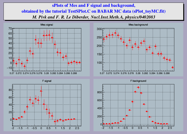
This tutorial illustrates the use of class TSPlot and of the sPlots method.

It is an example of analysis of charmless B decays, performed for BABAR. One is dealing with a data sample in which two species are present: the first is termed signal and the second background. A maximum Likelihood fit is performed to obtain the two yields N1 and N2 The fit relies on two discriminating variables collectively denoted y, which are chosen within three possible variables denoted Mes, dE and F. The variable which is not incorporated in y, is used as the control variable x. The distributions of discriminating variables and more details about the method can be found in the TSPlot class description

NOTE: This script requires a data file $ROOTSYS/tutorials/splot/TestSPlot_toyMC.dat.

Processing /mnt/build/workspace/root-makedoc-v610/rootspi/rdoc/src/v6-10-00-patches/tutorials/splot/TestSPlot.C...
estimated #of events in species 0 = 462.641575
estimated #of events in species 1 = 4957.409256
estimated #of events in species 0 = 490.068958
estimated #of events in species 1 = 4929.942571
estimated #of events in species 0 = 431.484129
estimated #of events in species 1 = 4988.519463
estimated #of events in species 0 = 420.453703
estimated #of events in species 1 = 4999.547303

#include "TSPlot.h"
#include "TTree.h"
#include "TH1.h"
#include "TCanvas.h"
#include "TFile.h"
#include "TPaveLabel.h"
#include "TPad.h"
#include "TPaveText.h"
#include "Riostream.h"
void TestSPlot()
{
   TString dir = gSystem->UnixPathName(__FILE__);
   dir.ReplaceAll("TestSPlot.C","");
   dir.ReplaceAll("/./","/");
   TString dataFile = Form("%sTestSPlot_toyMC.dat",dir.Data());
   //Read the data and initialize a TSPlot object
   TTree *datatree = new TTree("datatree", "datatree");
   datatree->ReadFile(dataFile,
                      "Mes/D:dE/D:F/D:MesSignal/D:MesBackground/D:dESignal/D:dEBackground/D:FSignal/D:FBackground/D",' ');
   TSPlot *splot = new TSPlot(0, 3, 5420, 2, datatree);
   //Set the selection for data tree
   //Note the order of the variables:
   //first the control variables (not presented in this example),
   //then the 3 discriminating variables, then their probability distribution
   //functions for the first species(signal) and then their pdfs for the
   //second species(background)
   splot->SetTreeSelection(
      "Mes:dE:F:MesSignal:dESignal:FSignal:MesBackground:"
      "dEBackground:FBackground");
   //Set the initial estimates of the number of events in each species
   //- used as initial parameter values for the Minuit likelihood fit
   Int_t ne[2];
   ne[0]=500; ne[1]=5000;
   splot->SetInitialNumbersOfSpecies(ne);
   //Compute the weights
   splot->MakeSPlot();
   //Fill the sPlots
   splot->FillSWeightsHists(25);
   //Now let's look at the sPlots
   //The first two histograms are sPlots for the Mes variable signal and
   //background. dE and F were chosen as discriminating variables to determine
   //N1 and N2, through a maximum Likelihood fit, and thus the sPlots for the
   //control variable Mes, unknown to the fit, was constructed.
   //One can see that the sPlot for signal reproduces the PDF correctly,
   //even when the latter vanishes.
   //
   //The lower two histograms are sPlots for the F variables signal and
   //background. dE and Mes were chosen as discriminating variables to
   //determine N1 and N2, through a maximum Likelihood fit, and thus the
   //sPlots for the control variable F, unknown to the fit, was constructed.
   TCanvas *myc = new TCanvas("myc",
   "sPlots of Mes and F signal and background", 800, 600);
   myc->SetFillColor(40);
   TPaveText *pt = new TPaveText(0.02,0.85,0.98,0.98);
   pt->SetFillColor(18);
   pt->SetTextFont(20);
   pt->SetTextColor(4);
   pt->AddText("sPlots of Mes and F signal and background,");
   pt->AddText("obtained by the tutorial TestSPlot.C on BABAR MC "
               "data (sPlot_toyMC.fit)");
   TText *t3=pt->AddText(
      "M. Pivk and F. R. Le Diberder, Nucl.Inst.Meth.A, physics/0402083");
   t3->SetTextColor(1);
   t3->SetTextFont(30);
   pt->Draw();
   TPad* pad1 = new TPad("pad1","Mes signal",0.02,0.43,0.48,0.83,33);
   TPad* pad2 = new TPad("pad2","Mes background",0.5,0.43,0.98,0.83,33);
   TPad* pad3 = new TPad("pad3", "F signal", 0.02, 0.02, 0.48, 0.41,33);
   TPad* pad4 = new TPad("pad4", "F background", 0.5, 0.02, 0.98, 0.41,33);
   pad1->Draw();
   pad2->Draw();
   pad3->Draw();
   pad4->Draw();
   pad1->cd();
   pad1->SetGrid();
   TH1D *sweight00 = splot->GetSWeightsHist(-1, 0, 0);
   sweight00->SetTitle("Mes signal");
   sweight00->SetStats(kFALSE);
   sweight00->Draw("e");
   sweight00->SetMarkerStyle(21);
   sweight00->SetMarkerSize(0.7);
   sweight00->SetMarkerColor(2);
   sweight00->SetLineColor(2);
   sweight00->GetXaxis()->SetLabelSize(0.05);
   sweight00->GetYaxis()->SetLabelSize(0.06);
   sweight00->GetXaxis()->SetLabelOffset(0.02);
   pad2->cd();
   pad2->SetGrid();
   TH1D *sweight10 = splot->GetSWeightsHist(-1, 1, 0);
   sweight10->SetTitle("Mes background");
   sweight10->SetStats(kFALSE);
   sweight10->Draw("e");
   sweight10->SetMarkerStyle(21);
   sweight10->SetMarkerSize(0.7);
   sweight10->SetMarkerColor(2);
   sweight10->SetLineColor(2);
   sweight10->GetXaxis()->SetLabelSize(0.05);
   sweight10->GetYaxis()->SetLabelSize(0.06);
   sweight10->GetXaxis()->SetLabelOffset(0.02);
   pad3->cd();
   pad3->SetGrid();
   TH1D *sweight02 = splot->GetSWeightsHist(-1, 0, 2);
   sweight02->SetTitle("F signal");
   sweight02->SetStats(kFALSE);
   sweight02->Draw("e");
   sweight02->SetMarkerStyle(21);
   sweight02->SetMarkerSize(0.7);
   sweight02->SetMarkerColor(2);
   sweight02->SetLineColor(2);
   sweight02->GetXaxis()->SetLabelSize(0.06);
   sweight02->GetYaxis()->SetLabelSize(0.06);
   sweight02->GetXaxis()->SetLabelOffset(0.01);
   pad4->cd();
   pad4->SetGrid();
   TH1D *sweight12 = splot->GetSWeightsHist(-1, 1, 2);
   sweight12->SetTitle("F background");
   sweight12->SetStats(kFALSE);
   sweight12->Draw("e");
   sweight12->SetMarkerStyle(21);
   sweight12->SetMarkerSize(0.7);
   sweight12->SetMarkerColor(2);
   sweight12->SetLineColor(2);
   sweight12->GetXaxis()->SetLabelSize(0.06);
   sweight12->GetYaxis()->SetLabelSize(0.06);
   sweight02->GetXaxis()->SetLabelOffset(0.01);
   myc->cd();
}

Authors: Anna Kreshuk, Muriel Pivc

Definition in file TestSPlot.C.